Spectracular Performance!

During the past 10 years Galaxy Zoo volunteers have done amazing work helping to classify the visual appearance (or “morphology”) of distant galaxies, which has enabled fantastic science that wouldn’t have been possible without your help. 

Morphology alone encodes a wealth information about the physical processes that drive the formation and ongoing evolution of galaxies, but we can learn even more if we analyze the spectrum of light they emit.

For the 100th Zooniverse project we designed the Galaxy Nurseries project to get your help analyzing galaxy spectra obtained by the Hubble Space Telescope (you can find many more details about Galaxy Nurseries on the main project research pages and this previous blog post).

If you participated in Galaxy Nurseries, then the data you analyzed were generated using a technique called slitless spectroscopy. In slitless spectroscopy all the light entering the HST aperture is dispersed (or split) into its separate frequencies before being projected directly into the telescope’s camera. Figure 1 illustrates a typically confusing result!

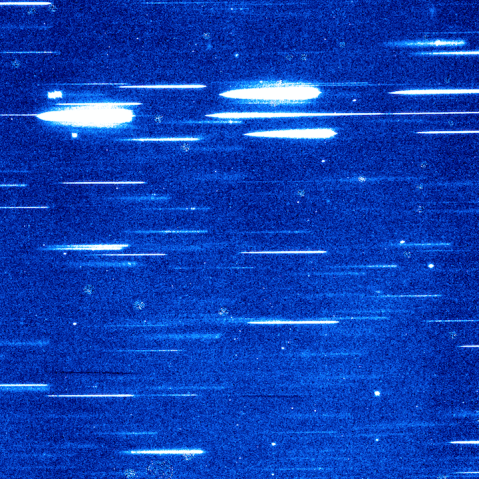
Figure 1: Example of data obtained by the Hubble Space Telescope using slitless spectroscopy.

Each bright horizontal streak in the image shown in Figure 1 is actually the spectrum of a different galaxy or star. Analyzing these data can be very tricky, especially when nearby galaxy spectra overlap and cross-contaminate each other. Automatic algorithms really struggle to reliably distinguish between spectral contamination and scientifically interesting features that are present in the spectra. This means that scientists almost aways need to visually inspect any features that are automatically detected in order to ensure that they are really there!

In Galaxy Nurseries, we asked volunteers to help with this verification process. We asked you to double-check over 27,000 automatically detected emission lines in galaxy spectra obtained by the WISP galaxy survey, labelling them as either real or fake. Even for professional astronomers and experienced Galaxy Zoo volunteers, verifying the presence of emission lines in slitless spectroscopic data can be very difficult. To help you discriminate between real and fake emission lines we showed you three different views of the data. Figure 2 shows an example of one of the Galaxy Nurseries subject images.

Figure 2: A Galaxy Nurseries subject showing a real emission line. The different panels show A) a 1-dimensional representation of the spectrum with the potential emission line marked ; B) a 2-dimensional “cutout” from the full slitless spectroscopic image, with the potential emission line and the expected extent of the galaxy spectrum marked; C) a direct image of the galaxy for which the spectrum was generated.

As well as the 1 dimensional spectrum shown in Figure 2 (Panel A), we also showed a “cutout” from the full slitless spectroscopic image, which isolated the target spectrum (Panel B), and a direct image of the galaxy that produced the spectrum (Panel C). The cutout in Panel B can be really useful for identifying contamination from adjacent spectra. For example, something that looks like a feature in the target spectrum might actually originate in an adjacent spectrum and would therefore appear slightly vertically off-centre in the 2-dimensional image.

Why is the direct image useful for spectroscopic analysis? Well, emission lines often appear like very slightly blurred images of the target galaxy at a specific position in the slitless spectrum. Look again at the emission line and the direct image in Figure 2. Can you see the similarity? If the shape of the automatically detected line feature in the slitless spectroscopic image doesn’t match the shape of the galaxy in the direct image, then this can indicate that the feature is just contamination masquerading as an emission line.

The response to Galaxy Nurseries was fantastic! Following its launch the project was completed in only 40 days, gathering 414,360 classifications (that’s 15 classifications per emission line) from 3003 volunteers. Huge thanks for everyones’ help! The results of the project were published in a Research Note, and the rest of this post summarizes what we learned.

Using the labels assigned to each potential emission line by galaxy zoo volunteers we computed the fraction of volunteers who classified the line and thought it was real (hereafter f_real). We wanted to compare the responses of the Galaxy Zoo volunteers with those of professional astronomers from the WISP survey team (WST). To do this, we divided the potential emission lines into two sets. The verified set contained emission lines that the WST thought were real and the vetoed set contained emission lines that the WST thought were fake. We assumed that the WST assessments were correct in the vast majority of cases, but this might not be completely accurate. Even professional astronomers make mistakes!

Figure 3 shows the distributions of f_real for the two sets of emission lines. The great news is that for the vast majority of lines that the WST thought were fake, over half of the volunteers agreed with them (i.e. f_real < 0.5). Similarly for most of the WST-verified set of line, the majority volunteers also labeled them as real. These results show us that Zooniverse and Galaxy Zoo volunteers are very capable when it comes to separating real emission lines from the fakes.

Figure 3: The distributions of f_real for sets of emission lines that were verified (blue) or vetoed (orange) by the WISP survey team.

What can we say about the lines for which the volunteers and the WST disagreed? Is there something about them that makes them particularly hard to classify? Well, it turns out that the answer is “yes”!

We computed two statistical metrics to quantify the level of agreement between the Zooniverse volunteers and the WST for a particular sample of the emission lines that were classified.

1. The sample purity is defined as the ratio between the number of true positives (for which both the volunteers and the WST believe the the line is real)  and the combined number of true positives and false positives (for which a feature labeled as fake by the WST was labeled as real by the volunteers). The purity tells us the fraction of lines in the sample that were labeled real by the volunteers that were also labeled as real by the WST. If volunteers don’t mislabel any fake lines as real then purity is 1.
2. The sample completeness is the ratio between the number of true positives and combined number of true positives and true negatives (for which the WST labeled the line as real, but the volunteer consensus was that the line was fake). The completeness tells us the fraction of lines in the sample that were labeled as real by the WST that were also labeled as real by the volunteers. If volunteers spot all the real lines identified by the WST then the completeness is 1.

Figure 4 plots purity and completeness as a function of f_real  and the emission line signal-to-noise ratio (S/N). Lines with higher S/N stand out more relative to the noise in the spectrum and should be easier to analyze for volunteers and the WST alike. Examining Figure 4 reveals that for subsets of candidate lines having f_real less than a particular threshold value (shown on the horizontal axis), the completeness values are higher for higher S/N. This indicates that spotting real lines is much easier when the features being examined are bright, which makes intuitive sense. On the other hand, higher purities can be achieved for similar threshold values of  f_real as the S/N value decreases, which indicates that volunteers are reluctant to label faint lines as real. At low S/N, sample purities as high as 0.8 can be achieved when only 50% of volunteers agreed that the corresponding emission lines were real. At higher S/N, volunteers become more confident, but also seem slightly more likely to identify noise and contaminants as real lines. This is probably a reflection of just how difficult the line identification task really is. Nonetheless, samples that are 70% pure can be selected by requiring a marginal majority of votes for real ( f_real value of at least 0.6), which is pretty impressive!

Figure 4: Sample purity (left) and completeness (right) plotted as a function of minimum f_real value for any potential line in the sample, and that line’s signal-to-noise ratio.

We can use the plots in Figure 4  to select samples that have desirable properties for scientific analysis. For example, if we want to be sure that we include 75% of all the real lines but we don’t mind a few fakes sneaking in, then we could choose  f_real = 0.5 which would give a completeness larger than 0.75 for all S/N values. However, if we choose f_real = 0.5, then the purity of our sample could be as low as 0.6 for high S/N, with about 40% of accepted lines being fake in reality.

The ability to extract very complete but impure emission line samples can be very useful. By selecting a sample that removes a sizable fraction of fakes from the automatically detected candidates, the number of potential lines that the WST need to visually inspect is dramatically reduced. It took the WST almost 5 months before each line in Galaxy Nurseries could be inspected by just two independent astronomers. By providing 15 independent classifications for each line, Zooniverse volunteers did the 8 times as much work in just 40 days! In the future, large-scale slitless spectroscopic surveys will be performed by new space telescopes like Euclid and WFIRST. These surveys will measure millions of spectra containing many millions of potential emission lines and individual science teams will simply not be able to visually inspect all of these lines. Eventually, deep learning algorithms may be able to succeed where current automatic algorithms fail. In the meantime, it is only with the help of Zooniverse and Galaxy Zoo volunteers that scientists will be able to exploit more than the tiniest fraction of the fantastic data that will soon arrive.