
Investigating How Type of Galactic Bar Impacts Bar Quenching
We are happy to announce the acceptance of the latest science team paper making use of Galaxy Zoo classifications (the image below is a link to the paper). Also see this list of all Galaxy Zoo Science Team Publications (which is mostly complete, usually!).
This work was led by (at the time) undergraduate student Petra Mengistu (since Fall 2024 in the PhD Program at UCSC). Petra started this work as an undergraduate, spending the summer of 2023 working at Oxford with the Galaxy Zoo science team there, and then returning to Haverford to continue the work for her undergraduate senior thesis. I’m writing this as a very proud (former) undergraduate supervisor today.
As the”Part II” in the title suggests, this work is a follow-on from previous work. Tobias Geron already wrote in detail about the first paper on the blog Slow Strong Bars Affect Their Hosts the Most which has a lot of the background needed to understand this follow-on result.
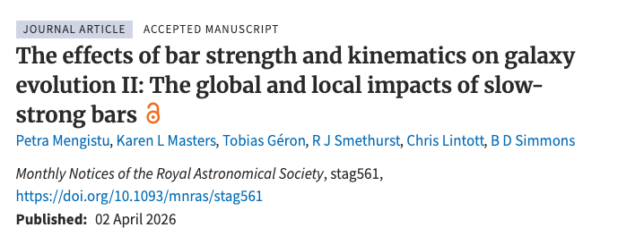
One fun thing we added was a look at the morphology of the ionized hydrogen around the bars in these galaxies (using data from the “MaNGA Survey”). This “Halpha” brightness can be traced by flux or “equivalent width” or EW (which is a measure of relative brightness compared to the stars you see in the normal images you are used to). It turns out this gas, which shows off where stars are currently forming in a galaxy – has a lot of different interesting shapes in barred galaxies, e.g. being found all along the bar, in rings or nodes.
The below image is a part of the sixth Figure in Petra’s paper.
There’s many more result in the paper, but I need to keep this blog post short for now.
Continuing to publish papers about bars in galaxies is also fun for me, as I’ve been working on trying to understand bars in galaxies using Galaxy Zoo classifications for well over a decade at this point. It’s great to see this work continuing with new samples and data and new understanding of the important role these structures play in stopping star formation in spiral galaxies. I wrote about bars for the blog “What’s all the Fuss about Bars in Galaxies” in 2015, or you can read this blog post from way back in 2010 (!) about our first Galaxy Zoo paper wondering “Do Bars Kill Galaxies”.
So thanks again for all the classifications. I’m excited for the future of this scientific area looking more at bars in the more distant universe (so looking back in time), which we already started with “Looking for Bars in Faraway Galaxies“, but I’m sure there will be much more to come.
Announcing the Galaxy Zoo JWST project!
We are thrilled to announce the launch of the Galaxy Zoo JWST project, with ~300,000 galaxy images from the COSMOS-Web survey taken with NASA’s James Webb Space Telescope (JWST)! We now need your help identifying the shapes of these galaxies by classifying them on Galaxy Zoo. These classifications will help scientists answer questions about how the shapes of galaxies have changed over time, and what caused these changes and why.
As we look at more distant objects in the Universe, we see them as they were billions of years ago because light takes time to travel to us. With JWST able to spot galaxies at greater distances than ever before, we’re seeing what galaxies looked like early in the Universe for the first time. The shape of the galaxies we see then tells us about what a galaxy has been through in its lifetime: how it was born, how and when it has formed stars, and how it has interacted with its neighbours. By looking at how galaxy shapes change with distance away from us, we can work out which processes were more common at different times in the Universe’s history.
Image credit: COSMOS-Web / Kartaltepe / Casey / Franco / Larson / RIT / UT Austin / CANDIDE.
Now, with data from JWST, we’re able to look deeper into the cosmos and further back in cosmic time than ever before, investigating the wild and wonderful ancestors of the Milky Way and the galaxies which surround us in today’s Universe. Thanks to the light collecting power of JWST, there are now over 300,000 images of galaxies on the Galaxy Zoo website that need your help to classify their shapes. If you’re quick, you may even be the first person to see the distant galaxies you’re asked to classify. You will be asked several questions, such as ‘Is the galaxy round?’, or ‘Are there signs of spiral arms?’. These classifications are not only useful for the scientific questions we want to answer now, but also as a training set for Artificial Intelligence (AI) algorithms. Without being taught what to look for by humans, AI algorithms struggle to classify galaxies. But together, humans and AI can accurately classify limitless numbers of galaxies.
We here at Galaxy Zoo have developed our own AI algorithm called ZooBot (see this previous blog post for more detail), which will sift through the JWST images first and label the ‘easier ones’ where there are many examples that already exist in previous images from the Hubble Space Telescope. When ZooBot is not confident on the classification of a galaxy, perhaps due to complex or faint structures, it will show it to users on Galaxy Zoo to get their human classifications, which will then help ZooBot to learn more.

You might also notice a slight difference to the classification interface for this project. Each image has two main colour versions available to help you see different features in the galaxy. Both of these colours images are built from the four COSMOSweb filters (F115W, F150W, F277W, and F444W) but with two different scalings. On the right the scaling is set to reveal bright central features more clearly, while the lefthand version should reveal fainter outskirts. You can also see the original four single filter images if you’d like in the flip book (see the two circles below the centre of the two images). By providing all of these images we’re hoping that it’ll be easier for volunteers to classify the images, and allow us to extract the most information about a galaxy from each image.
We’re really excited about this project on the team, not least because it’s been in the pipeline for a long time! We have had two team meetings at the International Space Science Institute (ISSI) in Bern, Switzerland over the past year in preparation for this launch, so it’s great to be finally at this point. We’re particularly excited though because of the science that will be made possible thanks to this project. Given JWST’s incredible sensitivity to light (thanks to that beautifully large mirror!), we’ll be able to classify the shapes of galaxies out to much greater distances than ever before. This means we can see further back in time in the Universe’s history to trace how the shapes of galaxies have changed earlier in cosmic time. We’ve already taken a look at your classifications from the pilot JWST project we ran on ~9000 galaxy images from the CEERS survey (another JWST galaxies survey, that’s smaller then COSMOS-Web that’s launching today) and with your help we found disk galaxies and galaxies with bars out to greater distances than ever before. So with even more JWST galaxies now on the site, all of us on the team are buzzing with excitement thinking of all the new discoveries coming our way soon.
If you do decide to take part: THANK YOU! We appreciate every single click. Join us and classify now.
Cosmic Disco: Help us characterize galaxy merger stages!
You have helped classify the morphologies of millions of galaxies through various Galaxy Zoo campaigns! Among those several millions are colliding galaxies (aka galaxy mergers) that are experiencing a significant change in their morphology and physical nature. Previously you have answered questions about the presence of disturbed morphological features (e.g., major or minor disturbance). As the process of galaxy merging can take several millions to a billion years, the merging galaxies we observe present to us in a plethora of configurations depending on their merging stage.

Identifying the stage of merging can help us better associate the impact of mergers to specific changes in the galaxy properties. An alternative approach is to use the disturbed morphological signatures (also called tidal features) as a proxy for merger staging. We are launching a new project Cosmic Disco: Characterizing Galaxy Collisions where you can help characterize the images containing mergers into objective categories.

We are looking forward to doing awesome science with your help! Happy Classifying!
Letting Things Slide: A New Trial Interface for Expressing Uncertainty
“How many spiral arms are in the image – is it two or three? Is that a disk viewed edge-on? I think so, but I’m not quite sure…” If you’ve interacted with Galaxy Zoo before, you may have asked yourself questions like these. Real galaxy images can be confusing. You may be uncertain!
Until now, you have always had to make a choice. There was no way to express uncertainty in your annotations. But now there is! Try it here.
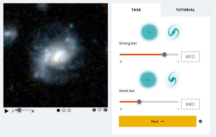
We are trialing a new experimental interface that lets you express your confidence in your annotations by dragging on a slider. This design is motivated by recent research indicating that we may be able to learn more, faster, by collecting annotator uncertainty [see this paper, this paper, this paper, this paper]. Allowing you to express your uncertainty by dragging a slider means that you – Zooniverse Friend – are providing more information with each click.
We believe this slider design might help us – through your support – discover more about galaxies, faster!
This is the second trial project we’re starting, adding to the Tags trial that Hayley introduced earlier on the blog. The big picture here is that we’re trying to think about how Galaxy Zoo could evolve in the coming years. As with any science project, we need to gather data and test our ideas.
Join in here and help us improve Galaxy Zoo.
We’ll run this trial for a short time – perhaps a couple of months – to gather your annotations and feedback. You can still use the current Galaxy Zoo that you know and (hopefully) love, at www.galaxyzoo.org.
Thank you for helping us,
Mike, Katie, and Ilia.
Planning for the Future of Galaxy Zoo – Science Team Meeting at ISSI
A large fraction of the Galaxy Zoo Science Team will be gathering at the International Space Science Institute (or ISSI) later this month to discuss the future of Galaxy Zoo, and in particular to work on the next phase of Galaxy Zoo now that there are large numbers of distant galaxies with publicly available JWST images.

This is part of a series of two funded meeting at ISSI that the Galaxy Zoo team was awarded with the goal of working on the next phases of Galaxy Zoo: JWST.
As the saying goes, if it isn’t broken don’t fix it. But also Galaxy Zoo has a tradition at being at the forefront of galaxy morphology techniques. So we want to use this meeting as an opportunity to spend some time reassessing the entire method that Galaxy Zoo pioneered back in 2007, when it was still a new idea to invite volunteers to participate in online image analysis. Our understanding of how to analyze your votes has evolved a lot over the last 17 years and across the more than 70 peer-reviewed publications the team has worked on. The status of machine learning methods for galaxy image analysis has also changed significantly, so it makes sense to reassess the most effective approach for humans and machines to collaborate on understanding the shapes and structures of galaxies.
The Galaxy Zoo science team has always been really international and distributed, with astronomers based all over the world. We are all really excited that ISSI has provided funding for us to have this rare gathering in person. We hope that by spending a week working together in person we can have some really productive discussions around the future of the project. We also have specific plans to work on getting the JWST images ready for your classifications as well as analyzing the results from the JWST:CEERS images you have already classified using our standard method.
As always we welcome volunteer input, not just via your classifications, but if you have opinions on what you would like to see in future versions of Galaxy Zoo, we invite you to share them on the Talk Forum.
Galaxy Zoo Upgrade: Better Galaxies, Better Science
Since I joined the team in 2018, citizen scientists like you have given us over 2 million classifications for 50,000 galaxies. We rely on these classifications for our research: from spiral arm winding, to merging galaxies, to star formation – and that’s just in the last month!
We want to get as much science as possible out of every single click. Your time is valuable and we have an almost unlimited pile of galaxies to classify. To do this, we’ve spent the past year designing a system to prioritise which galaxies you see on the site – which you can choose to access via the ‘Enhanced’ workflow.
This workflow depends on a new automated galaxy classifier using machine learning – an AI, if you like. Our AI is good at classifying boring, easy galaxies very fast. You are a much better classifier, able to make sense of the most difficult galaxies and even make new discoveries like Voorwerpen, but unfortunately need to eat and sleep and so on. Our idea is to have you and the AI work together.
The AI can guess which challenging galaxies, if classified by you, would best help it to learn. Each morning, we upload around 100 of these extra-helpful galaxies. The next day, we collect the classifications and use them to teach our AI. Thanks to your classifications, our AI should improve over time. We also upload thousands of random galaxies and show each to 3 humans, to check our AI is working and to keep an eye out for anything exciting.
With this approach, we combine human skill with AI speed to classify far more galaxies and do better science. For each new survey:
- 40 humans classify the most challenging and helpful galaxies
- Each galaxy is seen by 3 humans
- The AI learns to predict well on all the simple galaxies not yet classified
What does this mean in practice? Those choosing the ‘Enhanced’ workflow will see somewhat fewer simple galaxies (like the ones on the right), and somewhat more galaxies which are diverse, interesting and unusual (like the ones on the left). You will still see both interesting and simple galaxies, and still see every galaxy if you make enough classifications.
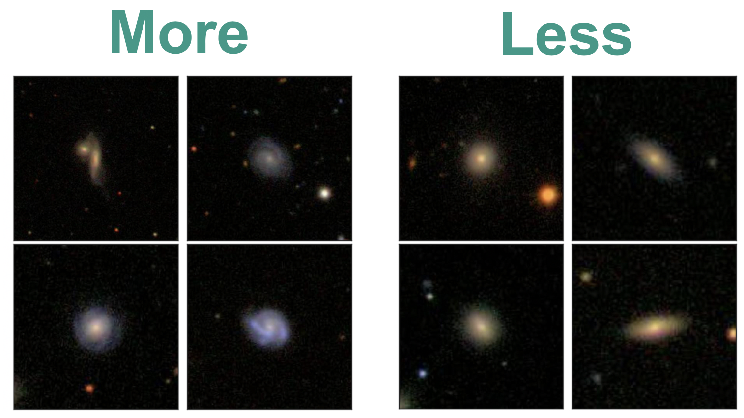
With our new system, you’ll see somewhat more galaxies like the ones on the left, and somewhat fewer like the ones on the right.
We would love for you to join in with our upgrade, because it helps us do more science. But if you like Galaxy Zoo just the way it is, no problem – we’ve made a copy (the ‘Classic’ workflow) that still shows random galaxies, just as we always have. If you’d like to know more, check out this post for more detail or read our paper. Separately, we’re also experimenting with sending short messages – check out this post to learn more.
Myself and the Galaxy Zoo team are really excited to see what you’ll discover. Let’s get started.
Scaling Galaxy Zoo with Bayesian Neural Networks
This is a technical overview of our recent paper (Walmsley 2019) aimed at astronomers. If you’d like an introduction to how machine learning improves Galaxy Zoo, check out this blog.
I’d love to be able to take every galaxy and say something about it’s morphology. The more galaxies we label, the more specific questions we can answer. When you want to know what fraction of low-mass barred spiral galaxies host AGN, suddenly it really matters that you have a lot of labelled galaxies to divide up.
But there’s a problem: humans don’t scale. Surveys keep getting bigger, but we will always have the same number of volunteers (applying order-of-magnitude astronomer math).
We’re struggling to keep pace now. When EUCLID (2022), LSST (2023) and WFIRST (2025ish) come online, we’ll start to look silly.

To keep up, Galaxy Zoo needs an automatic classifier. Other researchers have used responses that we’ve already collected from volunteers to train classifiers. The best performing of these are convolutional neural networks (CNNs) – a type of deep learning model tailored for image recognition. But CNNs have a drawback. They don’t easily handle uncertainty.
When learning, they implicitly assume that all labels are equally confident – which is definitely not the case for Galaxy Zoo (more in the section below). And when making (regression) predictions, they only give a ‘best guess’ answer with no error bars.
In our paper, we use Bayesian CNNs for morphology classification. Our Bayesian CNNs provide two key improvements:
- They account for varying uncertainty when learning from volunteer responses
- They predict full posteriors over the morphology of each galaxy
Using our Bayesian CNN, we can learn from noisy labels and make reliable predictions (with error bars) for hundreds of millions of galaxies.
How Bayesian Convolutional Neural Networks Work
There’s two key steps to creating Bayesian CNNs.
1. Predict the parameters of a probability distribution, not the label itself
Training neural networks is much like any other fitting problem: you tweak the model to match the observations. If all the labels are equally uncertain, you can just minimise the difference between your predictions and the observed values. But for Galaxy Zoo, many labels are more confident than others. If I observe that, for some galaxy, 30% of volunteers say “barred”, my confidence in that 30% massively depends on how many people replied – was it 4 or 40?
Instead, we predict the probability that a typical volunteer will say “Bar”, and minimise how surprised we should be given the total number of volunteers who replied. This way, our model understands that errors on galaxies where many volunteers replied are worse than errors on galaxies where few volunteers replied – letting it learn from every galaxy.
2. Use Dropout to Pretend to Train Many Networks
Our model now makes probabilistic predictions. But what if we had trained a different model? It would make slightly different probabilistic predictions. We need to marginalise over the possible models we might have trained. To do this, we use dropout. Dropout turns off many random neurons in our model, permuting our network into a new one each time we make predictions.
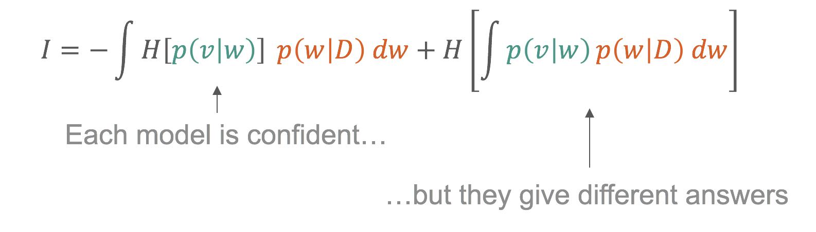
Below, you can see our Bayesian CNN in action. Each row is a galaxy (shown to the left). In the central column, our CNN makes a single probabilistic prediction (the probability that a typical volunteer would say “Bar”). We can interpret that as a posterior for the probability that k of N volunteers would say “Bar” – shown in black. On the right, we marginalise over many CNN using dropout. Each CNN posterior (grey) is different, but we can marginalise over them to get the posterior over many CNN (green) – our Bayesian prediction.

Read more about it in the paper.
Active Learning
Modern surveys will image hundreds of millions of galaxies – more than we can show to volunteers. Given that, which galaxies should we classify with volunteers, and which by our Bayesian CNN?
Ideally we would only show volunteers the images that the model would find most informative. The model should be able to ask – hey, these galaxies would be really helpful to learn from– can you label them for me please? Then the humans would label them and the model would retrain. This is active learning.
In our experiments, applying active learning reduces the number of galaxies needed to reach a given performance level by up to 35-60% (See the paper).
We can use our posteriors to work out which galaxies are most informative. Remember that we use dropout to approximate training many models (see above). We show in the paper that informative galaxies are galaxies where those models confidently disagree.
This is only possible because we think about labels probabilistically and approximate training many models.
What galaxies are informative? Exactly the galaxies you would intuitively expect.
- The model strongly prefers diverse featured galaxies over ellipticals
- For identifying bars, the model prefers galaxies which are better resolved (lower redshift)
This selection is completely automatic. Indeed, I didn’t realise the lower redshift preference until I looked at the images!
I’m excited to see what science can be done as we move from morphology catalogs of hundreds of thousands of galaxies to hundreds of millions. If you’d like to know more or you have any questions, get in touch in the comments or on Twitter (@mike_w_ai, @chrislintott, @yaringal).
Cheers,
Mike
One Million for Zooniverse – and One for Galaxy Zoo!

Galaxy Zoo started in 2007 because astronomers had 1,000,000 galaxies that needed to be sorted, classified, and examined. After the incredible response from the public, the zookeepers realized that this kind of problem wasn’t limited to galaxies, nor even just to astronomy, and the Zooniverse was born.
Now, seven actual years, close to 30 projects, more than 60 publications, and hundreds of years’ worth of human effort later, the Zooniverse has just registered its 1,000,000th volunteer. Given that Galaxy Zoo was the project that led to the creation of the Zooniverse, it seems fitting that its millionth citizen scientist joined to classify galaxies! That volunteer (whose identity we won’t divulge unless s/he gives us permission) joins over 400,000 others who have classified galaxies near and far. That number is 40% of the Zooniverse’s overall total — meaning that, while Galaxy Zoo has a large and vibrant community of volunteers and scientists, most people who join Zooniverse start off contributing to a different project. Many of them try other projects after their first: over on the Zooniverse blog Rob described the additions we’ve made to the Zooniverse Home area so that everyone who brought us to a million can see their own contribution “fingerprint” on the Zooniverse. Here’s what mine currently looks like:

The blue at the left is Galaxy Zoo; the dark orange is Snapshot Serengeti. #addict
Our millionth volunteer gets a cheesy prize (but hopefully useful: a Zooniverse tote bag and mug), and while we’d like to give that same prize to the 999,999 who came before him/her and to everyone who contributes to Galaxy Zoo and all Zooniverse projects, perhaps it’s more fitting that we say to everyone what’s really on our mind right now:

Galactic-Scale Gratitude. You all are awesome.
Evolutionary Paths In Galaxy Morphology: A Galaxy Zoo Conference

This week much of the team has been in Sydney, Australia, for the Evolutionary Paths In Galaxy Morphology conference. It’s a meeting centered largely around Galaxy Zoo, but it’s more generally about galaxy evolution, and how Galaxy Zoo fits into our overall (ever unfolding) picture of galaxy evolution.

There’s a lot to that legacy already, and it’s still being written.
The first talk of the conference was a public talk by Chris, fitting for a project that would not have been possible without public participation. Chris also gave a science talk later in the conference, summarizing many of the different results from Galaxy Zoo (and with a focus on presenting the results of team members who couldn’t be at the meeting). For me, Karen’s talk describing secular galaxy evolution and detailing the various recent results that have led us to believe “slow” evolution is very important was a highlight of Tuesday, and the audience questions seemed to express a wish that she could have gone on for longer to tie even more of it together. When the scientists at a conference want you to keep going after your 30 minutes are up, you know you’ve given a good talk.
In fact, all of the talks from team members were very well received, and over the course of the week so far we’ve seen how our results compare to and complement those of others, some using Galaxy Zoo data, some not. We’ve had a number of interesting talks describing the sometimes surprising ways the motions of stars and gas in galaxies compare with the visual morphologies. Where (and how bright) the stars and dust are in a galaxy doesn’t always give clues to the shape of the stars’ orbits, nor the extent and configuration of the gas that often makes up a large fraction of a galaxy’s mass.

Karen explains her simple and clear diagram showing different galaxy evolutionary processes.
This goes the other way, too: knowing the velocities of stars and gas in a galaxy doesn’t necessarily tell you what kinds of stars they are, how they got there, or what they’re doing right now. I suspect a combination of this kinematic information with the image information (at visual and other wavelengths) will in the future be a more often used and more powerful diagnostic tool for galaxies than either alone.
Overall, the meeting was definitely a success, and throughout the meeting we tried to keep a record of things so that others could keep up with the conference even if they weren’t able to attend. There was a lot of active tweeting about the conference, for example, and Karen and I took turns recording the tweets so that we’d have a record of each day of the Twitter discussion. Here those are, courtesy of Storify:
Also, remember at our last hangout when we said we’d have a hangout from Sydney? That proved a bit difficult, not just because of the packed meeting schedule but also because of bandwidth issues: overburdened conference and hotel wifi connections just aren’t really up to the task of streaming a hangout. We eventually found a place, but then it turned out there was construction going on next door, so instead of the sunny patio we had intended to run the hangout from we ended up in an upstairs bedroom to get as far away from the noise as possible. Ah, well. You can see our detailed discussion of how the meeting went below, including random contributions from the jackhammer next door (but only for the first few minutes):
(click here for the podcast version)
And now we’ll all return (eventually) to our respective institutions to reflect on the meeting, start work on whatever new ideas the conference discussions, talks and posters started brewing, and continue the work we had set aside for the past week. None of this is really as easy as it sounds; the best meetings are often the most exhausting, so it takes some time to recover. I asked our fearless leader Chris if he had a pithy statement to sum up his feeling of exhilarated post-meeting fatigue, and he took my keyboard and offered the following:
gt ;////cry;gvlbhul,kubmc ;dptfvglyknjuy,pt vgybhjnomk
I’m sure that, if any tears were shed, they were tears of joy. This is a great project and it’s only getting better.

Left to Right: Tom, Kevin, Bob, Amit, Ed, Chris S, Bill, Kyle, Chris L, Ivy, Brooke, Karen, Julie
Quench Boost: A How-To-Guide, Part 4
Now that we’ve been initiated into the cool waters of Tools (Part 1), we’ve compared our *own* galaxies to the rest of the post-quenched sample (Part 2), and we’ve put your classifications to use, looking for what makes post-quench galaxies special compared to the rest of the riff-raff (Part 3), we’re ready for Part 4 of the Quench ‘How-To-Guide’.
This segment is inspired by a post on Quench Talk in response to Part 3 of this guide. One of our esteemed zoo-ite mods noted:
There are more Quench Sample mergers (505) than Control mergers (245)… It seems to suggest mergers have a role to play in quenching star formation as well.
Whoa! That’s a statistically significant difference and will be a really cool result if it holds up under further investigation!
I’ve been thinking about this potential result in the context of the Kaviraj article, summarized by Michael Zevin at http://postquench.blogspot.com/. The articles finds evidence that massive post-quenched galaxies appear to require different quenching mechanisms than lower-mass post-quenched galaxies. I wondered — can our data speak to their result?
Let’s find out!
Step 1: Copy this Dashboard to your Quench Tools environment, as you did in Part 3 of this guide.
- This starter Dashboard provides a series of tables that have filtered the Control sample data into sources showing merger signatures and those that do not, as well as sources in low, mid, and high mass bins.
- Mass, in this case, refers to the total stellar mass of each galaxy. You can see what limits I set for each mass bin by looking at the filter statements under the ‘Prompt’ in each Table.
Step 2: Compare the mass histogram for the Control galaxies with merger signatures with the mass histogram for the total sample of Control galaxies.
- Click ‘Tools’ and choose ‘Histogram’ in the pop-up options.
- Choose ‘Control’ as the ‘Data Source’.
- Choose ‘log_mass’ as the x-axis, and limit the range from 6 to 12.
- Repeat the above, but choose ‘Control – Merging’ as the ‘Data Source’.
The result will look similar to the figure below. Can you tell by eye if there’s a trend with mass in terms of the fraction of Control galaxies with merger signatures?
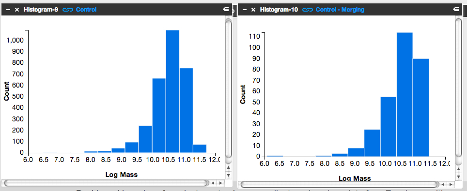
It’s subtle to see it in this visualization. Instead, let’s look at the fractions themselves.
Step 3: Letting the numbers guide us… Is there a higher fraction of Control galaxies with merger signatures at the low-mass end? At the high-mass end? Neither?
To answer this question, we need to know, for each mass bin, the fraction of Control galaxies that show merger signatures. I.e.,
![]()
Luckily, Tools can give us this information.
- Click on the ‘Control – Low Mass’ Table and scroll to its lower right.
- You’ll see the words ‘1527 Total Items’.
- There are 1527 Control galaxies in the low mass bin.
- Similarly, if you look in the lower right of the ‘Control – Merging – Low Mass’ Table, you’ll see that there are 131 galaxies in this category.
- This means that the merger fraction for the low mass bin is 131/1527 or 8.6%.
- Find the fraction for the middle and high mass bins.
Does the fraction increase or decrease with mass?
Step 4: Repeat the above steps but for the post-quenched galaxy sample.
You may want to open a new Dashboard to keep your window from getting too cluttered.
Step 5: How do the results compare for our post-quenched galaxies versus our Control galaxies? How can we best visualize these results?
- In thinking about the answer to this question, you might want to make a plot of mass (on the x-axis) versus merger fraction (on the y-axis) for the Control galaxies.
- On that same graph, you’d also show the results for the post-quenched galaxies.
- To determine what mass value to use, consider taking the median mass value for each mass bin.
- Determine this by clicking on ‘Tools’, choosing ‘Statistics’ in the pop-up options, selecting ‘Control – Low Mass’ as your ‘Data Source’, and selecting ‘Log Mass’ as the ‘Field’.
- This ‘Statistics’ Tool gives you the mean, median, mode, and other values.
- You could plot the results with pen on paper, use Google spreadsheets, or whatever plotting software you prefer. Unfortunately Tools, at this point, doesn’t provide this functionality.
It’d be awesome if you posted an image of your results here or at Quench Talk. We can then compare results, identify the best way to visualize this for the article, and build on what we’ve found.
You might also consider repeating the above but testing for the effect of choosing different, wider, or narrower mass bins. Does that change the results? It’d be really useful to know if it does.
