
Galaxy Zoo + Galaxy Zoo: 3D
Hi! I’m Tom, and I’m a PhD student at the University of Nottingham, doing some research to try to understand how spiral galaxies have grown and changed over their lifetimes. I’m especially interested in looking at how the spiral arms have been affecting the galaxy as a whole. I’ve recently finished up a paper in MNRAS in which I’ve been demonstrating a couple of new methods using some Galaxy Zoo data.
Amelia has already written [ https://blog.galaxyzoo.org/2018/07/17/finding-bars-in-galaxy-zoo-3d/ ] about how she is using the MaNGA survey [ https://www.sdss.org/surveys/manga/ ] to try to understand what’s happening in bars, so I won’t go into too much detail about this fantastic survey. I’ll just say that it’s part of the Sloan Digital Sky Survey, and for each of its sample of 10,000 galaxies, we have measurements of the spectrum at every position across the face of the galaxy.
MaNGA is really useful for trying to understand how galaxies have grown to their current size, because it is possible to get some sort of estimation of what kinds of stars are present in different locations of the galaxy. It’s a difficult thing to measure, so we can’t say exactly how many of every different type of star is present, but we can at least get a broad picture of the kinds of stellar ages and chemical enrichment (“metallicity”) in the stars. Astronomers have used these kinds of tools to measure the average age or metallicity of stars in different parts of galaxies, and found that in most spirals, the further out you go in the galaxy, the younger the stars are on average. The usual interpretation of this is that bulges tend to have formed first, and the disks have grown in size over time afterwards.

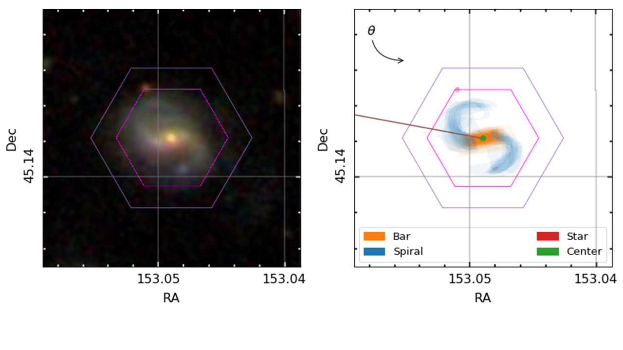
A MaNGA spiral galaxy. We can obtain information about the kinds of stars residing across the hexagonal area, which helps us understand how they’ve grown and evolved.
I’m really interested in trying to push this picture in two ways. Firstly, I’ve been trying to see what we can learn from looking at the general distribution of stars of different ages and metallicities – not just the average properties – at each location in the galaxy. Secondly, I think there is a lot of information that we risk ignoring by only looking at how things change with galactic radius. Spiral arms and the bar aren’t evenly distributed around the galaxy, so if we can see how the stellar properties change as we move around the galaxy, we should be able to measure what effect the spiral arms and bars have on the stars. The goal would be to try to confirm whether the most popular models of the nature of spiral arms and bars are correct or not.
To properly do this, we need to know exactly where the spiral arms and bars are in the MaNGA galaxies, so that we can see how the stars vary in these different regions. Enter Galaxy Zoo: 3D, where volunteers are asked to tell us where the different components are.
An example galaxy in MaNGA, where we’ve managed to split the galaxy into different stellar populations of different ages. Each frame shows where we find stars of a given age in this galaxy, starting from the oldest stars and finishing with the most recently formed stars. The colour denotes the mean metallicity of the stars, shown by the scale at the bottom.
All of this is what my most recent publication is about (read it in full at https://doi.org/10.1093/mnras/stz2204); we’ve shown that by combining the full spatial information available from MaNGA (augmented by Galaxy Zoo:3D) with the full distributions of the ages and metallicities of stars in each location, we can start to see some interesting things in the bar and spiral arms. It’s definitely best illustrated by an animation.
By splitting the age distributions up into different “time-slices”, we can create images of where stars of different ages are located in each of our MaNGA galaxies. Immediately from this one example, it’s obvious that there’s a lot of things going on here.
There are a few features in the animation that we’re not entirely convinced are real, but the main exciting things are that the spiral arms only show up in the youngest stars, and the bar grows and rotates as we move from older to younger stars. The growth of the bar is intriguing; this might be showing us how it formed. The bar changing with angle is even more exciting, and we think it shows us how quickly new-born stars become mixed and “locked” into the bar. The arms show what we should expect; spiral arms are areas of intense star formation, but over time the stars formed there will become mixed around the disk. We measured this effect by looking at what fraction of stars of each age are located in the volunteer-drawn spiral arms from Galaxy Zoo:3D.
This is really interesting, and highlights the power of combining large surveys like MaNGA with crowd-sourced information from the Zooniverse.
The next step is to do these kinds of things with more than just this one galaxy though. I’ve started looking at how these techniques can measure how fast the disks of spiral galaxies grew, using a large sample of spiral galaxies identified by Galaxy Zoo 2 volunteers. I’m also trying to measure how quickly stars get mixed away from spiral arms in different types of spiral galaxies. I have started to find some hints of some exciting results on both of these topics, which I would love to share in a future blog post if you’re interested.
We need volunteers to tell us where the spiral arms and bars are in galaxies, so that we can start to see what makes these regions special.
However, I’m currently limited in the number of galaxies with spiral arm regions identified by Galaxy Zoo:3D volunteers, so it would be really helpful if we could get some more! Understanding what makes spiral structure appear in disky galaxies is one of the unsolved problems in galaxy evolution and formation, and the clues to finding out might well lie in measuring how spiral arms affect the galaxy’s stars. Galaxy Zoo:3D will definitely be able to play a role in this! Help us out at https://www.zooniverse.org/projects/klmasters/galaxy-zoo-3d.
Bayesian View of Galaxy Evolution
The Universe is pretty huge, and to understand it we need to collect vast amounts of data. The Hubble Telescope is just one of many telescopes collecting data from the Universe. Hubble alone produces 17.5 GB of raw science data each week. That means since its launch to low earth orbit in April 1990, it’s collected roughly a block of data equivalent in size to 6 million mp3 songs! With the launch of NASA’s James Webb Telescope just around the corner – (a tennis court sized space telescope!), the amount of raw data we can collect from the Universe is going to escalate dramatically. In order to decipher what this data is telling us about the Universe we need to use sophisticated statistical techniques. In this post I want to talk a bit about a particular technique I’ve been using called a Markov-Chain-Monte-Carlo (MCMC) simulation to learn about galaxy evolution.
Before we dive in into the statistics let me try and explain what I’m trying to figure out. We can model galaxy evolution by looking at a galaxy’s star formation rate (SFR) over time. Basically we want know to how fast a particular galaxy is making stars at any given time. Typically, a galaxy has an initial constant high SFR then at a time called t quench (tq) it’s SFR decreases exponentially which is characterised by a number called tau. Small tau means the galaxy stops forming stars, or is quenched, more rapidly. So overall for each galaxy we need to determine two numbers tq and tau to figure out how it evolved. Figure 1 shows what this model looks like.

Figure 1: Model of a single galaxy’s SFR over time. Showing an initial high constant SFR, follow by a exponential quench at tq.
To calculate these two numbers, tq and tau, we look at the colour of the galaxy, specifically the UVJ colour I mentioned in my last post. We then compare this to a predicted colour of a galaxy for a specific value of tq and tau. The problem is that there are many different combinations of tq and tau, how to we find the best match for a galaxy? We use a MCMC simulation to do this.
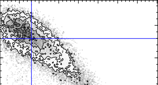
The first MC – Markov-Chain – just means an efficient random walk. We send “walkers” to have a look around for a good tq and tau, but the direction we send them to walk at each step depends on how good the tq and tau they are currently at is. The upshot of this is we quickly home in on a good value of tq and tau. The second MC – Monte Carlo – just picks out random values of tq and tau and tests how good they are by comparing the UVJ colours and our SFR model. Figure 2 shows a gif of a MCMC simulation of a single galaxy. The histograms shows the positions of the walkers searching the tq and tau space, and the blue crosshair shows the best fit value of tq and tau at every step. You can see the walkers homing in and settling down on the best value of tq and tau. I ran this simulation by running a modified version of the starpy code.
Figure 2: MCMC simulation for a single galaxy, pictured in the top right corner. Main plot shows density of walkers. Marginal histograms show 1D projections of walker densities. Blue crosshair shows best fit values of tq and tau at each step.
The maths that underpins this simulation is called Bayesian Statistics, and it’s quite a novel way of thinking about parameters and data. The main difference is that instead of treating unknown parameters as fixed quantities with associated error, they are treated as random variables described by probability distributions. It’s quite a powerful way of looking at the Universe! I’ve left all of the gory maths detail about MCMC out but if you’re interested an article by a DPhil student here at Oxford does are really good job of explaining it here.
So how does this all relate to galaxy morphology, and Galaxy Zoo classifications? I’m currently running the MCMC simulation showing in Figure 2 over the all the galaxies in the COSMOS survey. This is really cool because apart from getting to play with the University of Oxford’s super computer (544 cores!), I can use galaxy zoo morphology to see if the SFR of a galaxy over time is dependent on the galaxy’s shape, and overall learn what the vast amount of data I have says about galaxy evolution.
New images for Galaxy Zoo! Part 1 – DECaLS
We’re extremely excited to announce the launch of two new image sets today on Galaxy Zoo. Working with some new scientific collaborators over the past few months, we’ve been able to access data from two new sources. This blogpost will go into more details on where the images come from, what you might expect to see, and what scientific questions your classifications will help us answer. Part 2 of this post will discuss the other set of new images from the Illustris simulation.
The Dark Energy Camera Legacy Survey (DECaLS) is a public optical imaging project that follows up on the enormous, groundbreaking work done by the various versions of the SDSS surveys over the past decade. The aim of DECaLS is to use larger telescopes to get deeper images with significantly better data quality than SDSS, although over a somewhat smaller area. The science goals include studies of how both baryons (stars, gas, dust) and dark matter are distributed in galaxies, and particularly in measuring how those ratios change as a galaxy evolves. By adding morphology from Galaxy Zoo, our joint science teams will explore topics including disk structure in lower mass galaxies, better constraints on the rate at which galaxies merge, and gather more data on how the morphology relates to galaxy color and environment.
DECaLS observations use the Blanco telescope, which is located at CTIO in northern Chile at an altitude of 2200m (7200 ft). The telescope has a 4-m aperture mirror, giving it more than three times the collecting area of the SDSS telescope. The camera used for the survey is named DECam, a large-area and extremely sensitive instrument developed for a separate program called the Dark Energy Survey. The camera has 570 megapixels and covers a 2.2 degree field of view – more than 20 times the apparent size of the full moon! The combination of the exquisite dark-sky observing site, a sensitive wide-field camera, and larger telescope all combine to generate the new images, which will eventually include more than 140 million unique sources on the sky when DECaLS is finished.
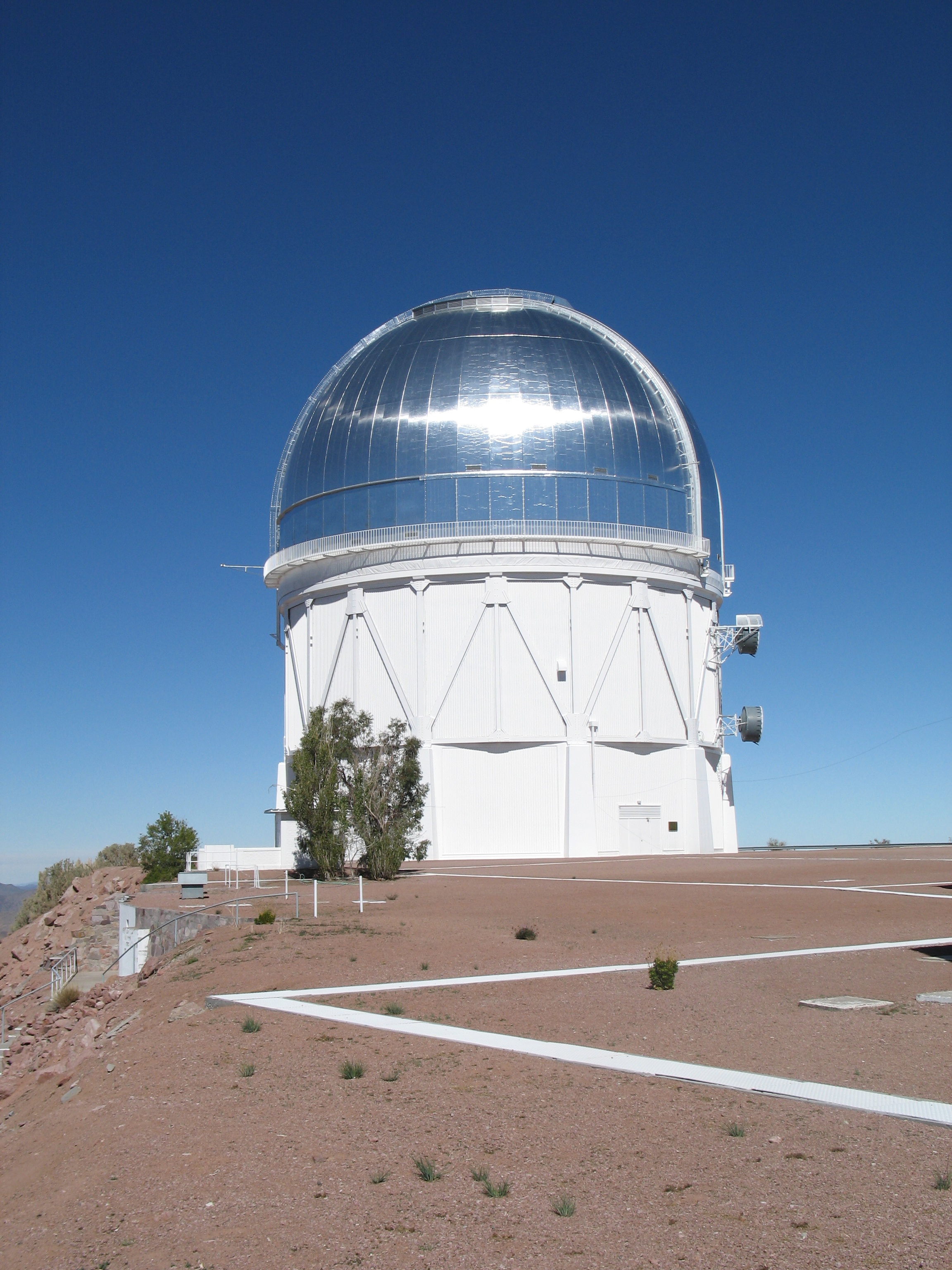
The Victor M. Blanco 4m telescope, located at CTIO in northern Chile, is carrying out the observations for the DECaLS survey. Image courtesy NOAO.
The DECaLS images in Galaxy Zoo are a smaller group taken from a catalog called the NASA-Sloan Atlas. We’re focusing on somewhat larger and brighter galaxies from the catalog. The reason is that although many of these galaxies have been classified in GZ already via their Sloan images, we’re particularly interested in measuring details like tidal tails from mergers, seeing fainter spiral structures, and separating galaxies that couldn’t be individually resolved in the Sloan data. Here’s a great example of a single galaxy in both SDSS and DECaLS – check out how much clearer the spiral arms are in the new images!

Left: an SDSS image of the galaxy J225336.34+000347.4. Right: a DECaLS image of the same galaxy.
Almost all of the morphology and classification tasks are the same as they were for the Sloan images, so it should be familiar to most of our users. If you have questions or want to discuss anything you see in the new images, please join the discussion with scientists and volunteers on Talk. As always, thanks for your help!
Making Radio Galaxies in a Computer
At a conceptual level the formation of radio galaxies is pretty simple. According to a basic picture first introduced in the 1970s, a supermassive black hole in the center of a galaxy generates a symmetric pair of oppositely directed, high speed jets or beams of hot, ionized gas as a by-product of energy released or stored from matter falling onto the black hole. Those jets drill holes in the atmosphere of the galaxy and then even far beyond, dumping energy, excavating cavities and possibly entraining gas into the jets and cavities along the way. The jets carry magnetic fields and high energy electrons. Those electrons, spiraling in the magnetic fields light up the jets and the cavities they excavate in the radio band through a process called synchrotron emission.
While calculations based on this cartoon picture can correctly predict a few properties of radio galaxies, anyone who has looked at the images in Radio Galaxy Zoo can see that there must be a whole lot more to the story. Radio galaxies at best have only a rough bilateral symmetry with respect to their host galaxies. Furthermore, no two radio galaxies look alike, and most look pretty complicated; some could only be described as messy. In fact, the physics of radio galaxy formation is really very complex for a whole bunch of reasons that range from inherent instabilities in the dynamics of a fast jet, to the reality that the jets are not steady at the source. Furthermore, the surrounding environments are themselves messy, dynamic and sometimes even violent. All of these influences have impact on the appearances of radio galaxies.
The other side of the coin is that, if they can be understood, these complications may improve opportunities to decipher both the formation processes of the jets as well as the conditions that control their development and dissipation as they penetrate their environments. One part of piecing this puzzle together is expanding our awareness of all the things radio galaxies do, as well as when and where they do what they do. That’s what Radio Galaxy Zoo is about.
On the other hand, to go beyond the cartoon picture of what we see we also have to develop much more sophisticated and realistic models of the phenomena. This is very challenging. Because the detailed physics is so complex (messy!), astronomers have come to depend increasingly on large computer simulations that solve equations for gas dynamics with magnetic fields and high energy electrons. Pioneering gas dynamical simulations of jets in the 1980s already played an important role in confirming the value of the jet paradigm and helped to refine it soon after it was introduced.
Those early simulations were, however, seriously limited by available computer power and computational methods. In important ways the structures they made did not really look much like actual radio galaxies. At best they were too grainy. At worst important physics had to be left out, including the processes that actually produce the radio emission. This made it hard to know exactly how to compare the simulations with real radio galaxies. Thankfully, rapid improvements in both of those areas have led recently to much more realistic and detailed simulations that are starting to look more like the real thing and can be used to better pin down what is actually going on.
Our group at the University of Minnesota has been involved for some years now in pushing forward the boundaries of what can be learned about radio galaxies from simulations. I illustrate below some of the lessons we have learned from these simulations and some of the complex radio galaxy environments that it is now possible to explore through simulations. Each of these simulations was part of the work carried out by a student as part of their PhD training.
The jets responsible for radio galaxy formation propagate at speeds that can be a significant fraction of the speed of light. They are almost certainly supersonic. These properties lead to several related behaviors that are illustrated in Figure 1. It turns out that the flows within such a jet tend periodically to expand and then to contract. As they do so they form a sequence of shocks along the jet. These are visible in the figure. The jet also creates a sonic boom or bow shock in front as it moves forward. A close look at the jet in this figure also reveals that the jet actually does not remain straight as it moves forward. The end of the jet turns out to be unstable, so soon after launch begins to ‘flap’ or wobble. As a result the end of the jet tends to jump around, enlarging the area of impact on the ambient medium.

Figure 1: Shock waves in a simulated high speed jet propagating from the left end of the box. Since the jet is driving supersonically through its ambient medium, it also has created a bow shock (sonic boom) in the ambient medium on the far right.
Many radio galaxies form inside clusters of galaxies, where the ambient medium is highly non-uniform and stirred up as a result of its own, violent formation. This distorts and bends the radio structures. At the same time the energy and momentum deposited by the jets creates cavities in the cluster gas that lead to dark holes in the thermal X-ray emission of the cluster. Figure 2 illustrates some of these behaviors for a simulated radio galaxy formed at the center of a cluster. Even though the source of the radio galaxy is at rest, there are fast gas motions in the cluster gas that obviously deflect the radio galaxy jets. ‘Mock’ radio images representing synchrotron emission by high energy electrons in the magnetic field carried by the jets are shown on the right in the figure at two times. At the same two times mock images of thermal X-rays are shown to the left. The X-ray images have been processed to exaggerate the dark cavities produced by the jets. Note that each image spans about 700 kpc or 2 million light years.

Figure 2: Simulation of radio galaxy formation in a cluster of galaxies that was extracted from a separate simulation of galaxy cluster formation. Mock observations of thermal X-rays (left) and radio synchrotron emission (right) are shown at two times after a pair of oppositely directed jets formed in the cluster center.
Quite a few radio galaxies in clusters are not made by galaxies anchored in the cluster center, but are hosted by galaxies moving through the cluster. This is especially common in clusters that are in the process of merging with another cluster. In that case the host galaxy can be moving very fast, and even supersonically with respect to its local, ambient medium. Then the radio jets can be very strongly deflected into ‘tails’ by an effective cross wind and eventually disrupted. Figure 3 illustrates the mock synchrotron emission from such a simulated radio galaxy. The abruptness of jet bending depends on the relative speed of the jet with respect to its internal sound speed and the relative speed of the host galaxy through its ambient medium with respect to the sound speed of that medium. So, when strongly bent jets are seen in a radio galaxy it is a strong clue that the motion of the galaxy is supersonic in relation to its environment. When multiple tailed radio galaxies are found in a given cluster it provides potentially valuable information about the dynamical condition of the cluster, since a relaxed cluster ought not to have many galaxies moving at supersonic speeds through the cluster gas.

Figure 3: Mock synchrotron image of a simulated radio galaxy embedded in a supersonic cross wind. The two jets have bent into downstream, turbulent tails .
Even more complex motions between the host galaxies and the ambient gas are possible. Those can sometimes lead to really exotic-looking radio structures. One beautiful example of this is the radio source 3C75 in the merging cluster Abell 400. Evidently two massive galaxies have become gravitationally bound into a binary system with a separation of about 7 kpc. The orbital period should be around 100 Myr. The pair also appears to be moving together supersonically through the ambient medium. Each of those galaxies has formed radio jets. If it were not for the binary the expected outcome might resemble the situation pictured in Figure 3. However, the binary motions cause each of the two galaxies to oscillate in its motion and this causes the radio jets to develop more complex, twisted shapes before they disrupt into tails. Figure 4 illustrates a preliminary effort to simulate this dynamics. The image on the right shows the real 3C75, where pink is the radio emission (VLA) and blue is thermal X-rays (Chandra). The image on the left traces the distribution of gas expelled by each of the two galaxies in the binary system. This simulation seems to capture the general character of the dynamical situation responsible for 3C75.

Figure 4: Right-the radio galaxy 3C75 as seen in the radio (pink) and associated thermal X-rays from the cluster Abell 400 (blue). Left-Simulated jets from a binary pair of galaxies intended to mimic the dynamics of 3c75.
From this short set of simulation results it ought to be clear why many different kinds of radio galaxy structures are expected to form. It also ought to be apparent that we need better catalogs of what behaviors do exist in nature in order to see how to focus our simulation efforts and to establish what are the most important dynamical conditions in radio galaxy formation.
GZ: Quench data update
Since finishing the classifications for the GZ: Quench project, many of our volunteers have been analyzing that consensus data using the tools at tools.galaxyzoo.org. We made a few changes to the site earlier this week, and I’d like to describe them and talk about how it might affect your work on the project.
First, a quick reminder of how the data is presented. As most of you probably remember, the classification process on GZ: Quench (and all GZ projects since GZ2) is what we call a “decision tree”. We begin with a broad question on morphology (ie, “Is this galaxy smooth, or does it have features or a disk?”) for the volunteer to answer. We then ask more specific follow-up questions that depend on the previous answers. For example – if you said the galaxy doesn’t have any spiral arms, it doesn’t make sense for us to then ask you how many arms there are – it doesn’t apply to this galaxy! So, out of 11 potential questions covering galaxy morphology, a single classifier will only answer a subset (between 4 and 9) of them. Here’s a flowchart of the decision tree for GZ: Quench — it’s an interesting exercise to look at it and work out how many unique morphologies you could sort galaxies into by going through the tree.

Flowchart of the morphology decision tree for GZ: Quench
So, why this discussion? When we added the data to the Tools website, we added a label in each category that gave the most common response to that question. For example, under “Arm tightness”, you could see that all galaxies were either “Tight”, “Medium”, or “Loose”. However, this is problematic when you’re trying to analyze data and compare different sets of galaxies. For smooth (or elliptical) galaxies, though, this arm classification is the result of very few votes (or even none) — they don’t represent the majority of classifications, and thus we really shouldn’t be including them when trying to compare what makes a medium-wound vs. a loosely-wound spiral.
The solution we’ve adopted has been to edit the data on Tools — questions whose answers don’t apply to the consensus morphology (eg, spiral arms in a smooth galaxy, or the roundness of a spiral) are now blank. This means that if you look at the average color or size of any of these morphology properties, you’re now truly comparing similar groups of objects (apples to apples). Including other galaxies in earlier samples likely introduced a significant amount of bias – the science team thinks that this will largely help to address that.
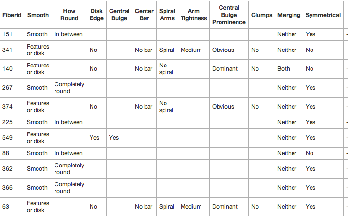
Example of the new GZ: Quench classification set in Tools
What does this mean for your analysis? Most of your old Dashboards and results should still work and remain valid results. For any work where you were analyzing morphological details (especially for spiral structure), though, we encourage you to revisit these and run them again on the new, filtered dataset. Please keep posting any questions you have on Talk, and we’ll answer them as soon as we can. Good luck!
Using Galaxy Zoo Classifications – a Casjobs Example
As Kyle posted yesterday, you can now download detailed classifications from Galaxy Zoo 2 for more than 300,000 galaxies via the Sloan Digital Sky Survey’s “CasJobs” – which is a flexible SQL-based interface to the databases. I thought it might be helpful to provide some example queries to the data base for selecting various samples from Galaxy Zoo.
This example will download what we call a volume limited sample of Galaxy Zoo 2. Basically what this means is that we attempt to select all galaxies down to a fixed brightness in a fixed volume of space. This avoids biases which can be introduced because we can see brighter galaxies at larger distances in a apparent brightness limited sample like Galaxy Zoo (which is complete to an r-band magnitude of 17 mag if anyone wants the gory details).
So here it is. To use this you need to go to CasJobs (make sure it’s the SDSS-III CasJobs and not the one for SDSS-I and SDSS-II which is a separate page and only includes SDSS data up to Data Release 7), sign up for a (free) account, and paste these code bits into the “Query” tab. I’ve included comments in the code which explain what each bit does.
 -- Select a volume limited sample from the Galaxy Zoo 2 data set (which is complete to r=17 mag).
 -- Also calculates an estimate of the stellar mass based on the g-r colours.
 -- Uses DR7 photometry for easier cross matching with the GZ2 sample which was selected from DR7.
 -- This bit of code tells casjobs what columns to download from what tables.
 -- It also renames the columns to be more user friendly and does some maths
 -- to calculate absolute magnitudes and stellar masses.
 -- For absolute magnitudes we use M = m - 5logcz - 15 + 5logh, with h=0.7.
 -- For stellar masses we use the Zibetti et al. (2009) estimate of
 -- M/L = -0.963+1.032*(g-i) for L in the i-band,
 -- and then convert to magnitude using a solar absolute magnitude of 4.52.
 select g.dr7objid, g.ra, g.dec,
 g.total_classifications as Nclass,
 g.t01_smooth_or_features_a01_smooth_debiased as psmooth,
 g.t01_smooth_or_features_a02_features_or_disk_debiased as pfeatures,
 g.t01_smooth_or_features_a03_star_or_artifact_debiased as pstar,
 s.z as redshift,
 s.dered_u as u, s.dered_g as g, s.dered_r as r, s.dered_i as i, s.dered_z as z, s.petromag_r,
 s.petromag_r - 5*log10(3e5*s.z) - 15.0 - 0.7745 as rAbs,
 s.dered_u-s.dered_r as ur, s.dered_g-s.dered_r as gr,
 (4.52-(s.petromag_i- 5*log10(3e5*s.z) - 15.0 - 0.7745))/2.5 + (-0.963 +1.032*(s.dered_g-s.dered_i)) as Mstar
-- This tells casjobs which tables to select from.
 from DR10.zoo2MainSpecz g, DR7.SpecPhotoAll s
-- This tells casjobs how to match the entries in the two tables
 where
 g.dr7objid = s.objid
 and
 -- This is the volume limit selection of 0.01<z<0.06 and Mr < -20.15
 s.z < 0.06 and s.z > 0.01
 and (s.petromag_r - 5*log10(3e5*s.z) - 15 - 0.7745) < -20.15
--This tells casjobs to put the output into a file in your MyDB called gz2volumelimit
 into MyDB.gz2volumelimit
Once you have this file in your MyDB, you can go into it and make plots right in the browser. Click on the file name, then the “plot” tab, and then pick what to plot. Colour-magnitude diagrams are interesting – to make one, you would plot “rabs” on the X-axis and “ur” (or “gr”) on the yaxis. There will be some extreme outliers in the colour, so put in limits (for u-r a range of 1-3 will work well). The resulting plot (which you will have to wait a couple of minutes to be able to download) should look something like this:

Or if you want to explore the GZ classifications, how about plotting “psmooth” (which is approximately the fraction of people viewing a galaxy who thought it was smooth) against the colour.
That plot would look something like this:
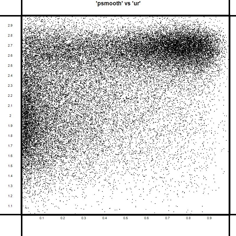
Which reveals the well known relationship between colour and morphology – that redder galaxies are much more likely to be ellipticals (or “smooth” in the GZ2 language) than blue ones.
You can learn more about SQL and the many things you could do with CasJobs at the Help Page (and then come back and tell me how simple my query example was!).
This example only downloads the very first answer from the GZ2 classification tree – there’s obviously a lot more in there to explore.
(Note that at the time of posting the DR10 server seemed to be struggling – perhaps over demand. I’m sure it will be fixed soon and this will then work.)
Good Things come at the same time
AAS meeting update!
The last 24 hours have been good for Zoo team member Bill Keel (@ngc3314) is based at the University of Alabama. Not only did his University football team win some sort of championship (they all look the same to Europeans) last night, but the Hubble Space Telescope observed the final Voorwerpje in our approved programme! That means Bill was probably glued to the TV and downloading and reducing the data at the same time!

He’ll add the reduced image to his poster at the AAS meeting, so if you want to see the image, come join us at the poster tomorrow! He may also blog it some time later, but for the FIRST look, you’ll have to come to the poster! There may be chocolates too….
The poster is: 339.47. HST Imaging of Giant Ionized Clouds Around Fading AGN, up all of Wednesday from 9-6.
New Dataset from Galaxy Zoo!
We’ve posted a new data set here: http://data.galaxyzoo.org/#agn
This sample is presented in the Galaxy Zoo 1 paper on AGN host galaxies (Schawinski et al., 2010, ApJ, 711, 284). It is a volume-limited sample of galaxies (0.02 < z < 0.05, M_z < -19.5 AB) with emission line classifications, stellar masses, velocity dispersions and GZ1 morphological classifications. When using this sample, please cite Schawinski et al. 2010 and Lintott et al. 2008, 2011.
Download here: http://galaxy-zoo-1.s3.amazonaws.com/schawinski_GZ_2010_catalogue.fits.gz
Column definitions are as follows:
- OBJID – SDSS object ID
- RA, DEC – RA and Dec in J2000
- REDSHIFT – SDSS spectroscopic redshift
- GZ1_MORPHOLOGY – Galaxy Zoo 1 morphology according to the Land et al. (2008) “clean” criterion. GZ_morphology is an integer where 1-early type, 4-late type, 0-indeterminate, 3-merger
- BPT_CLASS – 0-no emission lines, 1-SF, 2-Composite, 3-Seyfert and 4-LINER (see Schawinski et al. 2010 for details)
- U,G,R,I,Z -SDSS modelMag extinction corrected but not k-corrected
- SIGMA, SIGMA_ERR – Stellar velocity dispersion measured using GANDALF
- LOG_MSTELLAR – log of stellar mass
- L_O3 – Extinction-corrected [OIII] luminosity
Preethi's Cross-Eyed Galaxy

Remember this object from back in February? It turned up in a paper that I was reading today, going by the name of Preethi’s cross-eyed galaxy.
The paper, by Preethi Nair (now in Italy) and Roberto Abraham from the University of Toronto, is going to be really important as we analyze data from Zoo 2 and from Galaxy Zoo : Hubble. As part of her thesis work, Preethi examined over 14000 galaxies – twice each, to check for consistency (!) – in order to produce the largest detailed morphological catalogue in existence. We’ll be comparing your results to hers, and hopefully showing that the classifications for the other 280,000 or so galaxies in Zoo 2 are as reliable as her 14,000.
Or at least, that’s the theory. In practice I’ve spent the day trying to be sure I understand which of her objects match which of ours. But seeing an old friend – albeit with a new name – crop up still made me smile.
Zoo 1 data set free
Hi all
It’s taken longer than it should have done – more than three years since the launch of the site – but the data from the original galaxy zoo is now available.

The paper describing the data set was only accepted by the journal yesterday, but we were confident enough after an earlier report to go ahead and make it public. The data can also be downloaded in a variety of formats from our site, or via Casjobs.
The data set is slightly updated from our previous efforts; while we’ve been busy with Galaxy Zoo, the good people of the Sloan Digital Sky Survey produced a new data release which included more spectra, allowing us to estimate biases for more galaxies than ever before.
We’ve had a lot of fun exploring this data set, and we hope that by making it available to all other astronomers then they will make use of your classifications too.
Knowing the Zoo, I wouldn’t be too surprised to see something interesting come from any of you who wanted to have a play – feel free to download and dig in, and let us know how you get on. Meanwhile, the team are working hard on Zoo 2, and hopefully it won’t take as long before that data set too is ready to go.
