
Evolutionary Paths In Galaxy Morphology: A Galaxy Zoo Conference

This week much of the team has been in Sydney, Australia, for the Evolutionary Paths In Galaxy Morphology conference. It’s a meeting centered largely around Galaxy Zoo, but it’s more generally about galaxy evolution, and how Galaxy Zoo fits into our overall (ever unfolding) picture of galaxy evolution.

There’s a lot to that legacy already, and it’s still being written.
The first talk of the conference was a public talk by Chris, fitting for a project that would not have been possible without public participation. Chris also gave a science talk later in the conference, summarizing many of the different results from Galaxy Zoo (and with a focus on presenting the results of team members who couldn’t be at the meeting). For me, Karen’s talk describing secular galaxy evolution and detailing the various recent results that have led us to believe “slow” evolution is very important was a highlight of Tuesday, and the audience questions seemed to express a wish that she could have gone on for longer to tie even more of it together. When the scientists at a conference want you to keep going after your 30 minutes are up, you know you’ve given a good talk.
In fact, all of the talks from team members were very well received, and over the course of the week so far we’ve seen how our results compare to and complement those of others, some using Galaxy Zoo data, some not. We’ve had a number of interesting talks describing the sometimes surprising ways the motions of stars and gas in galaxies compare with the visual morphologies. Where (and how bright) the stars and dust are in a galaxy doesn’t always give clues to the shape of the stars’ orbits, nor the extent and configuration of the gas that often makes up a large fraction of a galaxy’s mass.

Karen explains her simple and clear diagram showing different galaxy evolutionary processes.
This goes the other way, too: knowing the velocities of stars and gas in a galaxy doesn’t necessarily tell you what kinds of stars they are, how they got there, or what they’re doing right now. I suspect a combination of this kinematic information with the image information (at visual and other wavelengths) will in the future be a more often used and more powerful diagnostic tool for galaxies than either alone.
Overall, the meeting was definitely a success, and throughout the meeting we tried to keep a record of things so that others could keep up with the conference even if they weren’t able to attend. There was a lot of active tweeting about the conference, for example, and Karen and I took turns recording the tweets so that we’d have a record of each day of the Twitter discussion. Here those are, courtesy of Storify:
Also, remember at our last hangout when we said we’d have a hangout from Sydney? That proved a bit difficult, not just because of the packed meeting schedule but also because of bandwidth issues: overburdened conference and hotel wifi connections just aren’t really up to the task of streaming a hangout. We eventually found a place, but then it turned out there was construction going on next door, so instead of the sunny patio we had intended to run the hangout from we ended up in an upstairs bedroom to get as far away from the noise as possible. Ah, well. You can see our detailed discussion of how the meeting went below, including random contributions from the jackhammer next door (but only for the first few minutes):
(click here for the podcast version)
And now we’ll all return (eventually) to our respective institutions to reflect on the meeting, start work on whatever new ideas the conference discussions, talks and posters started brewing, and continue the work we had set aside for the past week. None of this is really as easy as it sounds; the best meetings are often the most exhausting, so it takes some time to recover. I asked our fearless leader Chris if he had a pithy statement to sum up his feeling of exhilarated post-meeting fatigue, and he took my keyboard and offered the following:
gt ;////cry;gvlbhul,kubmc ;dptfvglyknjuy,pt vgybhjnomk
I’m sure that, if any tears were shed, they were tears of joy. This is a great project and it’s only getting better.

Left to Right: Tom, Kevin, Bob, Amit, Ed, Chris S, Bill, Kyle, Chris L, Ivy, Brooke, Karen, Julie
We got (some) observing time!
Great news everybody!
We applied for radio observations with the e-MERLIN network of radio telescopes in the UK. The e-MERLIN network can link up radio dishes across the UK to form a really, really large radio telescope using the interferometry technique. Linking all these radio dishes means you get the resolution equivalent to a country-sized telescope. You don’t alas get the sensitivity, as the collecting area is still just that of the sum of the dishes you are using.

The e-MERLIN network (from http://www.e-merlin.ac.uk) of radio telescopes.
Our proposal was to observe the Voorwerpjes. We wanted to take a really high resolution look at what the black holes are doing right now by looking for nuclear radio jets. The Voorwerpjes, like their larger cousin, Hanny’s Voorwerp, tell us that black holes can go from a feeding frenzy to a starvation diet in a short time scale (for a galaxy, that is). We really want to see what happens to the central engine of the black hole as that happens. There’s a suspicion that as the black hole stops gobbling matter as fast as it can, it starts “switching state” and launches a radio jet that starts putting a lot of kinetic energy (think hitting the galaxy with a hammer).
So, we want to look for such radio jets in the Voorwerpjes. We asked for a LOT of time, and the e-MERLIN time allocation committee approved our request…
… partially. Rather than giving us the entire time, they gave us time for just one source to prove that we can do the observations, and that they are as interesting as we claimed. So, we’re trying to decide which target to pick (argh! so hard).
Quench Boost: A How-To-Guide, Part 4
Now that we’ve been initiated into the cool waters of Tools (Part 1), we’ve compared our *own* galaxies to the rest of the post-quenched sample (Part 2), and we’ve put your classifications to use, looking for what makes post-quench galaxies special compared to the rest of the riff-raff (Part 3), we’re ready for Part 4 of the Quench ‘How-To-Guide’.
This segment is inspired by a post on Quench Talk in response to Part 3 of this guide. One of our esteemed zoo-ite mods noted:
There are more Quench Sample mergers (505) than Control mergers (245)… It seems to suggest mergers have a role to play in quenching star formation as well.
Whoa! That’s a statistically significant difference and will be a really cool result if it holds up under further investigation!
I’ve been thinking about this potential result in the context of the Kaviraj article, summarized by Michael Zevin at http://postquench.blogspot.com/. The articles finds evidence that massive post-quenched galaxies appear to require different quenching mechanisms than lower-mass post-quenched galaxies. I wondered — can our data speak to their result?
Let’s find out!
Step 1: Copy this Dashboard to your Quench Tools environment, as you did in Part 3 of this guide.
- This starter Dashboard provides a series of tables that have filtered the Control sample data into sources showing merger signatures and those that do not, as well as sources in low, mid, and high mass bins.
- Mass, in this case, refers to the total stellar mass of each galaxy. You can see what limits I set for each mass bin by looking at the filter statements under the ‘Prompt’ in each Table.
Step 2: Compare the mass histogram for the Control galaxies with merger signatures with the mass histogram for the total sample of Control galaxies.
- Click ‘Tools’ and choose ‘Histogram’ in the pop-up options.
- Choose ‘Control’ as the ‘Data Source’.
- Choose ‘log_mass’ as the x-axis, and limit the range from 6 to 12.
- Repeat the above, but choose ‘Control – Merging’ as the ‘Data Source’.
The result will look similar to the figure below. Can you tell by eye if there’s a trend with mass in terms of the fraction of Control galaxies with merger signatures?
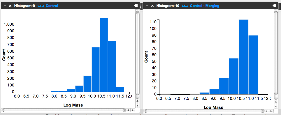
It’s subtle to see it in this visualization. Instead, let’s look at the fractions themselves.
Step 3: Letting the numbers guide us… Is there a higher fraction of Control galaxies with merger signatures at the low-mass end? At the high-mass end? Neither?
To answer this question, we need to know, for each mass bin, the fraction of Control galaxies that show merger signatures. I.e.,
![]()
Luckily, Tools can give us this information.
- Click on the ‘Control – Low Mass’ Table and scroll to its lower right.
- You’ll see the words ‘1527 Total Items’.
- There are 1527 Control galaxies in the low mass bin.
- Similarly, if you look in the lower right of the ‘Control – Merging – Low Mass’ Table, you’ll see that there are 131 galaxies in this category.
- This means that the merger fraction for the low mass bin is 131/1527 or 8.6%.
- Find the fraction for the middle and high mass bins.
Does the fraction increase or decrease with mass?
Step 4: Repeat the above steps but for the post-quenched galaxy sample.
You may want to open a new Dashboard to keep your window from getting too cluttered.
Step 5: How do the results compare for our post-quenched galaxies versus our Control galaxies? How can we best visualize these results?
- In thinking about the answer to this question, you might want to make a plot of mass (on the x-axis) versus merger fraction (on the y-axis) for the Control galaxies.
- On that same graph, you’d also show the results for the post-quenched galaxies.
- To determine what mass value to use, consider taking the median mass value for each mass bin.
- Determine this by clicking on ‘Tools’, choosing ‘Statistics’ in the pop-up options, selecting ‘Control – Low Mass’ as your ‘Data Source’, and selecting ‘Log Mass’ as the ‘Field’.
- This ‘Statistics’ Tool gives you the mean, median, mode, and other values.
- You could plot the results with pen on paper, use Google spreadsheets, or whatever plotting software you prefer. Unfortunately Tools, at this point, doesn’t provide this functionality.
It’d be awesome if you posted an image of your results here or at Quench Talk. We can then compare results, identify the best way to visualize this for the article, and build on what we’ve found.
You might also consider repeating the above but testing for the effect of choosing different, wider, or narrower mass bins. Does that change the results? It’d be really useful to know if it does.
Quench Boost: A How-To-Guide, Part 3
I’m very happy to be posting again to the How-To-Guide. We’ve made a number of updates to Quench data and Quench Tools. Before I launch into Part 3 of the Guide, here are the recent updates:
- The classification results for the 57 control galaxies that needed replacements have been uploaded into Quench Tools.
- We’ve applied two sets of corrections to the galaxies magnitudes: the magnitudes are now corrected for both the effect of extinction by dust and the redshifting of light (specifically, the k-correction).
- We’ve uploaded the emission line characteristics for all the control galaxies.
- We’ve uploaded a few additional properties for all the galaxies (e.g., luminosity distances and star formation rates).
- We corrected a bug in the code that mistakenly skipped galaxies identified as ‘smooth with off-center bright clumps’.
In Part 1 of this How-To-Guide to data analysis within Quench, you learned how to use Tools and were introduced to the background literature about post-quenched galaxies and galaxy evolution.
In Part 2 you used Tools to compare results from galaxies *you* classified with the rest of the post-quenched galaxy sample.
In Part 3 we’re going to use the results from the classifications that you all provided to see if there’s anything different about the post-quenched galaxies that have merged or are in the process of merging with a neighbor, and those that show no merger signatures.
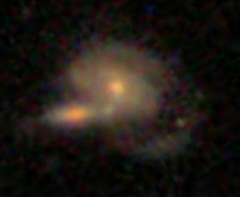
The figure below is of one of my favorite post-quenched galaxies with merger signatures. Gotta love those swooping tidal tails!
Let’s get started!
Step 1: Because of the updates to Tools, first clear your Internet browser’s cache, so it uploads the latest Quench Tools data.
Step 2: Copy my starter dashboard with emission line ratios ready for play.
- Open my Dashboard and click ‘Copy Dashboard’ in the upper right. This way you can make changes to it.
- In this Dashboard, I’ve uploaded the post-quenched galaxy data.
- I also opened a Table, just as you did in Part 2 of this How-To-Guide. I called the Table ‘All Quench Table’.
- In the Table, notice how I’ve applied a few filters, by using the syntax:
filter .’Halpha Flux’ > 0
- This reduces the table to only include sources that fulfill those criteria.
- Also notice that I’ve created a few new columns of data, just as you did in Part 2, by using the syntax:
field ‘o3hb’, .’Oiii Flux’/.’Hbeta Flux’
- That particular syntax means that I took the flux for the doubly ionized oxygen emission line ([0III]) and divided it by the flux in one of the Hydrogen emission lines (Hbeta).
- This ratio and the ratio of [NII]/Halpha are quite useful for identifying Active Galactic Nuclei (AGN).
- It’d be really interesting if we find that AGN play a role in shutting off the star formation in our post-quenched galaxies. A major question in galaxy evolution is whether there’s any clear interplay between merging, AGN activity, and shutting off star formation.
Step 3: Create the BPT diagram using the ratios of [OIII]/Hb and [NII]/Ha.
- BPT stands for Baldwin, Phillips, and Terlevich (1981), among the first articles to use these emission line ratios to identify AGN. Check out the GZ Green Peas project’s use of the BPT diagram.
- Click on ‘Tools’. Choose ‘Scatter plot’ in the pop-up options.
- In the new Scatterplot window, choose ‘All Quench Table’ as your ‘Data Source’.
- For the x-axis, choose ‘logn2ha’. For the y-axis, choose ‘logo3hb’.
- Adjust the min/max values so the data fits nicely within the window, as shown in the figure below.
- Remember that you can click on the comb icon in the upper-left of the plot to make the menu overlay disappear.
- Do you notice the two wings of the seagull in your plot? The left-hand wing is where star forming galaxies reside (potentially star-bursting galaxies) while the right-hand wing is where AGN reside. Our post-quenched sample of galaxies covers both wings.

Step 4: Compare the BPT diagram for post-quenched galaxies with and without signatures of having experienced a merger.
- To do this, you’ll need to first create two new tables, one that filters out merging galaxies and the other that filters out non-merging galaxies.
- Click on ‘Tools’. Choose ‘Table’ in the pop-up options.
- In the new Table window, choose ‘All Quench Table’ as the ‘Data Source’. Notice how this new table already has all the new columns that were created in the ‘All Quench Table’. That makes our life easier!
- Look through the column names and find the one that says ‘Merging’. Possible responses are ‘Neither’, ‘Merging’, ‘Tidal Debris’, or ‘Both’.
- Let’s pick out just the galaxies with no merger signatures.
- Under ‘Prompt’ type:
filter .Merging = ‘Neither’
- If you scroll to the bottom of the Table, you’ll notice that you now have only 2191 rows, rather than the original 3002.
- Call this Table ‘Non-Mergers Table’ by double clicking on the ‘Table-4’ in the upper-left of the Table and typing in the new name.
- Now follow the instructions from Step 3 to create a BPT scatter plot for your post-quenched galaxies with no merger signatures. Be sure to choose ‘Non-Mergers Table’ as the ‘Data Source’.
- You might notice that this plot looks pretty similar to the plot for the full post-quenched galaxy sample, just with fewer galaxies.
What about post-quenched galaxies that show signatures of merger activity? Do they also show a similar mix of star forming galaxies and AGN?
- To find out, create a new Table, but this time under ‘Prompt’ type:
filter .Merging != ‘Neither’
- The ‘!=’ syntax stands for ‘Not’, which means this filter picks out galaxies that had any other response under the ‘Merging’ column (i.e, tidal tails, merger, both). Notice how there are 505 sources in this Table.
- Now create a BPT scatter plot for your ‘Mergers Table’.
- Make sure this plot has a similar xmin,xmax,ymin,ymax as your other plots to ensure a fair comparison.
- You might also compare histograms of log(NII/Ha) for the different subsamples.
What do you find? Do you notice the difference? What could this be telling us about our post-quenched galaxies?!
Before you get too carried away in the excitement, it’s a good idea to compare the post-quenched galaxy sample BPT results against the control galaxy sample.
This comparison with the control sample will tell you whether this truly is an interesting and unique result for post-quenched galaxies, or something typical for galaxies in general. You might consider doing this in a new Dashboard, as I have, to keep things from getting too cluttered. In that new Dashboard, click ‘Data’, choose ‘Quench’ in the pop-up options, and choose ‘Quench Control’ as your data to upload. Now repeat Steps 1-4.
Do you notice any differences between your control galaxy and post-quenched galaxy sample results? What do you think this tells us about our post-quenched galaxies?
Stay tuned for Part 4 of this How-To-Guide. I’d love to build from your results from this stage, so definitely post the URLs for your Dashboards here or within Quench Talk and your questions and comments.
More Galaxies, More Clicks, More Science!
Just a quick update: recently we brought some of our high-redshift (i.e., very distant) galaxies out of retirement. There’s enough going on in these galaxies that having more clicks from you will really help tease out the nuances of the various features and make the classifications even better.
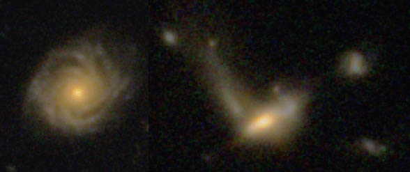
How would you classify these?
So, for those of you who noticed you hadn’t seen many CANDELS galaxies recently, well, you’re about to see a few more. I can’t promise they’ll always be easy to classify, but I hope they’ll at least be an interesting puzzle. As ever, thank you for your classifications!
What is a Galaxy? …the return
The first time I gave a public talk, I spent an hour describing why galaxy classification is fundamentally important to the study of the Universe, the origins of Galaxy Zoo, the amazing response of the volunteers and the diverse results from their collective classifications of a million galaxies near and far. I showed many gorgeous galaxy images, a few dark matter simulations and even a preview of the Hubble image of Hanny’s Voorwerp.
As I finished my talk and the Q&A began, I braced myself for the inevitably interesting and challenging questions (I seem to get a lot of questions about black holes and spacetime).
A brief pause, and then the first question echoed from somewhere in the darkened auditorium: …”What’s a galaxy?”
Oops. Apparently I’d forgotten that little detail at the start of the talk. So I described a typical galaxy (if there is such a thing): a collection of stars, gas, dust, dark matter, all gravitationally bound together. Then I made a joke about scientists forgetting to define their terms, and we moved on to the next raised hand.
Turns out, though, it’s not such an easy question. Even though my casual definition works fine for most galaxies, it’s not at all an agreed-upon standard. We’ve discussed this on the blog before, and even in the short time (astronomically speaking) since Karen wrote that very nice post, more work has been done to find galaxies that push the boundaries and force us to re-think what it really means to be a galaxy.

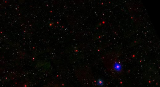
The circled stars (plus a lot of dark matter you can’t see) are Segue 1, one of the smallest galaxies we know about. To read more on this, click the image.
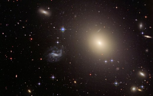
So, spurred by a very broad interpretation of a question left for us in the comments on the post announcing this hangout, we decided to re-visit the discussion, covering the various properties a galaxy must have, should have, could have, and can’t have. We discussed the smallest galaxies, found by counting and measuring each of their individual stars. We discussed the biggest, brightest galaxies in the universe, living in rich environments and grown fat by eating other galaxies. And everything in between.
Note: when we talk about Segue 1 and 2, I say that these galaxies are unique because they have low mass-to-light ratios. Despite the pause that indicated I was trying to keep from inverting numerator and denominator… that’s exactly what I did. The galaxies have very few stars compared to the amount of dark matter in them, so their mass is high and their light is low, so their mass-to-light ratios are high. Oops (again)!
Next GZ Hangout: 3rd of September, 3 pm GMT
The hangouts have returned from a midsummer hiatus! Our next hangout will be Tuesday, September 3rd, at 3 pm GMT. That’s 8 am PDT, 11 am EDT, 4 pm BST, 5 pm CET, 6 pm CAT. Unfortunately I think that’s 11 pm in Japan and midnight in Sydney, but hopefully we’ll have a hangout at a different time very soon!
Just before the hangout we’ll update this post with the embedded video, so you can watch it live from here. If you’re watching live and want to jump in on Twitter, please do! we use a term you’ve never heard without explaining it, please feel free to use the Jargon Gong by tweeting us. For example: “@galaxyzoo GONG dark matter halo“.
In the meantime, please feel free to leave a question in the comments below. See you soon!
Update: read a summary of the Hangout here: What is a Galaxy?… the Return
