
Explaining clustering statistics we use to study the distribution of Galaxy Zoo galaxies
I’ve used some statistical tools to analyze the spatial distribution of Galaxy Zoo galaxies and to see whether we find galaxies with particular classifications in more dense environments or less dense ones. By “environment” I’m referring to the kinds of regions that these galaxies tend to be found: for example, galaxies in dense environments are usually strongly clustered in groups and clusters of many galaxies. In particular, I’ve used what we call “marked correlation functions,” which I’ve found are very sensitive statistics for identifying and quantifying trends between objects and their environments. This is also important from the perspective of models, since we think that massive clumps of dark matter are in the same regions as massive galaxy groups.
We’ve mainly used them in two papers, where we analyzed the environmental dependence of morphology and color and where we analyzed the environmental dependence of barred galaxies. These papers have been described a bit in this post andthis post. We’ve also had other Galaxy Zoo papers about similar subjects, especially this paper by Steven Bamford and this one by Kevin Casteels.
What I loved about these projects is that we obtained impressive results that nobody else had seen before, and it’s all thanks to the many many classifications that the citizen scientists have contributed. These statistics are useful only when one has large catalogs, and that’s exactly what we had in Galaxy Zoo 1 and 2. We have catalogs with visual classifications and type likelihoods that are ten times as large as ones other astronomers have used.
What are these “marked correlation functions”, you ask? Traditional correlation functions tell us about how objects are clustered relative to random clustering, and we usually write this as 1+ ξ. But we have lots of information about these galaxies, more than just their spatial positions. So we can weight the galaxies by a particular property, such as the elliptical galaxy likelihood, and then measure the clustering signal. We usually write this as 1+W. Then the ratio of (1+W)/(1+ξ), which is the marked correlation function M(r), tells us whether galaxies with high values of the weight are more dense or less dense environments on average. And if 1+W=1+ξ, or in other words M=1, then the weight is not correlated with the environment at all.

First, I’ll show you one of our main results from that paper using Galaxy Zoo 1 data. The upper panel shows the clustering of galaxies in the sample we selected, and it’s a function of projected galaxy separation (rp). This is something other people have measured before, and we already knew that galaxies are clustered more than random clustering. But then we weighted the galaxies by the GZ elliptical likelihood (based on the fraction of classifiers identifying the galaxies as ellipticals) and then took the (1+W)/(1+ξ) ratio, which is M(rp), and that’s shown by the red squares in the lower panel. When we use the spiral likelihoods, the blue squares are the result. This means that elliptical galaxies tend to be found in dense environments, since they have a M(rp) ratio that’s greater than 1, and spiral galaxies are in less dense environments than average. When I first ran these measurements, I expected kind of noisy results, but the measurements are very precise and they far exceeded my expectations. Without many visual classifications of every galaxy, this wouldn’t be possible.

Second, using Galaxy Zoo 2 data, we measured the clustering of disc galaxies, and that’s shown in the upper panel of the plot above. Then we weighted the galaxies by their bar likelihoods (based on the fractions of people who classified them as having a stellar bar) and measured the same statistic as before. The result is shown in the lower panel, and it shows that barred disc galaxies tend to be found in denser environments than average disc galaxies! This is a completely new result and had never been seen before. Astronomers had not detected this signal before mainly because their samples were too small, but we were able to do better with the classifications provided by Zooites. We argued that barred galaxies often reside in galaxy groups and that a minor merger or interaction with a neighboring galaxy can trigger disc instabilities that produce bars.
What kinds of science shall we use these great datasets and statistics for next? My next priority with Galaxy Zoo is to develop dark matter halo models of the environmental dependence of galaxy morphology. Our measurements are definitely good enough to tell us how spiral and elliptical morphologies are related to the masses of the dark matter haloes that host the galaxies, and these relations would be an excellent and new way to test models and simulations of galaxy formation. And I’m sure there are many other exciting things we can do too.
…One more thing: if you’re interested, you’re welcome to check out my own blog, where I occasionally write posts about citizen science.
Radio interferometry, Fourier transforms, and the guts of radio interferometry (Part 1)
Today’s post comes from Dr Enno Middelberg and is the first part of two explaining in more detail about radio interferometry and the techniques used in producing the radio images in Radio Galaxy Zoo.
I have written in an earlier post about the basic idea of how to increase the resolution of a radio telescope: use many telescopes, separated by kilometers, and observe the same object with all. Here is a little more information about how this works.
At the very heart of an interferometer is the van Cittert-Zernike theorem: it essentially states that the degree of similarity of the electric field at two locations is a measure of the Fourier transform of the sky brightness distribution. Now that’s a big bite to swallow, but let me explain it in less confusing words: the electric field is all we can measure – radio waves are electromagnetic waves, and radio telescopes are sensitive to the electric field. Now we can build a radio telescope in a way that it produces as its output a voltage which is proportional to the electric field which the antenna receives from, e.g., a galaxy. Much of the signal will be noise from our own Milky Way, the atmosphere and the electronics which amplify the feeble signals, but a tiny little bit of the signal will be caused by radio waves from space, and both antennas will receive a little bit of these. Now suppose we have two telescopes separated by 1 km or so, and both telescopes produce such voltages which contain a little bit of this signal. The voltages are digitised and the two data streams are fed into a correlator. The correlator is a computer which takes the two data streams and calculates their correlation coefficient, which is an indicator for their similarity. If the two data streams have nothing in common (for example, because an unexperienced PhD student pointed the two antennas in different directions 🙂 ) then the correlation coefficient will be zero, which is to say that they are not similar at all. However, if the two telescopes point at the same source, the data streams will have a few bits in common, and the correlator spits out a correlation coefficient which is not zero. This is our measurement!
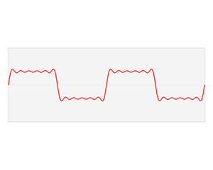
Now that we’ve that out of the way, we need to talk about Fourier transforms. The van Cittert-Zernike theorem states that the correlation coefficient is a measure for the Fourier transform of the sky brightness. Now what is a Fourier transform? The Fourier transform is an ingenious way of representing a mathematical function with a sum of sine and cosine functions. That is, if I take a large number of sine and cosine functions with various (but carefully selected!) frequencies and amplitudes, then their sum will be an accurate representation of another function, for example a square wave or a sawtooth. Check out the Wikipedia page on Fourier series (which are related to Fourier transforms, but easier to understand), which has a number of nice animations to illustrate this, such as this one:
![]()
You can also play with Paul Falstad’s Java applet to see how to construct functions using sine and cosine waves interactively – very instructive! In part 2 of this post I will explain how astronomers use 2D Fourier transforms to assemble images of the radio sky.
Radio Galaxy Zoo is now available in Chinese!
We’re pleased to announce that Radio Galaxy Zoo has been
translated to traditional character Chinese. Many thanks
to the Zooniverse’s Chris Snyder for getting all the technical
things set up for the translation to go live and Mei-Yin Chou
at Academia Sinica’s Institute of Astronomy & Astrophysics
(ASIAA) for helping verifying the translation. What follows
is an announcement describing Radio Galaxy Zoo and the translation
in traditional character Chinese and then in English: 電 波星系動物園[中 文版]歡 迎你的加入!在此我們欣然宣佈本計畫中文版開始啟用。
感謝中央研究院天文及天文物理研究所 Dr. Meg Schwamb (Meg是 參與Planet
Hunters 和Planet Four計 畫的科學家)以 及天文推廣團隊成員黃珞文協助,
將英文內容翻譯轉換為繁體中文。在 許多星系核心深處其實隱匿著一些超大質量的黑洞,
其質量往往為太陽的幾億倍,這些大黑洞雖然無法直接看得到,不過有
時仍可看得到從星系核心噴出的巨大噴流。由 電波波段看到的天空和在「可見光」
波段所看到的(可見的意思就是人類肉眼所看得到的),此兩種景象有時大異其 趣。
譬如,有些星系中心根本沒有電波輻射發出,但卻會向外噴發電波噴流,
或有時這些噴流的外觀是筆直的直線,有時卻 是一團、只有單邊而非雙邊對稱、
甚或是彎曲弧線等。藉由大型全天電波普查觀測計畫,我們取得了各式各樣多達幾十萬個
電波噴流和團塊影像,它們需要和所屬的宿主星系做成匹配。因 此,我們邀請你加入我們的行列,
來認識一個「從未曾見過」的宇宙,也借用您眼所見的,協助辨識電波波段之噴流(或細絲),
再將它 們和紅外圖像進行比較及匹 配,這麼一來,在你的協助下,
噴流和宿主星系間本來付之闕如的關聯 性,未來將可建立成形。 http://radio.galaxyzoo.org/?lang=zh_twWelcome to Radio Galaxy Zoo (Chinese)! It is with great
pleasure that we announce the launch of the Chinese version
of our project. We are very grateful to Dr Meg Schwamb
(from Planet Hunters and Planet Four) and Lauren Huang from
Academia Sinica’s Institute of Astronomy & Astrophysics
(ASIAA) for their help with translating our project from
English to traditional Chinese characters. Supermassive black holes (~several hundred million times
the mass of our Sun) lie deep in the cores of many galaxies.
And though we cannot directly see these black holes, we do
sometimes see the huge radio jets originating from the galaxy
cores. Galaxies in the radio sky can look quite different from
the one seen in the optical wavelengths by instruments such
as our own eyes. Some galaxies do not have any central radio
emission but only radio jet(s) emanating outwards. Sometimes
these jets are straight but at other times, they can be blobby,
one-sided or bent. With very large all-sky radio surveys, we
have many hundreds of thousands of radio jets and blobs that
need to be matched to their host galaxies. Therefore we invite you to see the Universe as you have never
seen before and help us map the radio sky by matching the radio
jets and filaments to the galaxies (as seen in the infrared images) from
whence they came. http://radio.galaxyzoo.org/?lang=zh_tw

Remarkable Discoveries Underway – Citizen Scientists fire up Radio Galaxy Zoo
Radio Galaxy Zoo participants have been swamping the Science Team with an incredible number of interesting objects via Talk. Many of these are challenging our understanding of how radio galaxies work, both at their launching sites in supermassive black holes, and in the ways that the ejected jets of radio plasma interact with their environment.
We’ll be highlighting some of these curious discoveries in subsequent blogs, but here’s a recently found one that’s just “too good to be true.”
Today, we know that a galaxy’s redshift (the measure of how fast it is moving away from us — we use z = velocity/speed of light, approximately) is an excellent indicator of distance. This is due to the overall expansion of the Universe. So a galaxy with z=0.049 is moving away at 14,700 km/s, and is located about 650 million light years away, while a galaxy with z=0.26 is moving at about 89,000 km/s and is 3 billion light years away.
How, then, could two such galaxies each be a source of radio emission which appear to be connected with a thin radio filament? That’s exactly what the following picture shows, where the optical picture, in green, is from the Sloan Digital Sky Survey (SDSS) , and the purple structure, outlined in white contours, is radio emission from the Faint Images of the Radio Sky at Twenty cm (FIRST, from the Very Large Array).
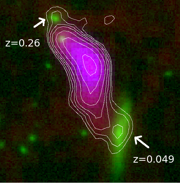
A cosmic coincidence
Radio Galaxy Zoo participants have looked at approximately 40,000 systems so far, so in such a large collection, this unusual object is likely just a coincidence, rather than some failure in our understanding of cosmic expansion. However, it would be nice to get some higher resolution radio images to see what the structure really looks like.
If you haven’t given Radio Galaxy Zoo a try yet – please join us at http://radio.galaxyzoo.org. We’re finding all kinds of fascinating new structures, while simultaneously creating a large database matching up radio emission with the supermassive black holes from which they were born.
