
New Images on Galaxy Zoo, Part 1
We’re delighted to announce that we have some new images on Galaxy Zoo for you to classify! There are two sets of new images:
1. Galaxies from the CANDELS survey
2. Galaxies from the GOODS survey
The general look of these images should be quite familiar to our regular classifiers, and we’ve already described them in many previous posts (examples: here, here, and here), so they may not need too much explanation. The only difference for these new images are their sensitivities: the GOODS images are made from more HST orbits and are deeper, so you should be able to better see details in a larger number of galaxies compared to HST.

Comparison of the different sets of images from the GOODS survey taken with the Hubble Space Telescope. The left shows shallower images from GZH with only 2 sets of exposures; the right shows the new, deeper images with 5 sets of exposures now being classified.
The new CANDELS images, however, are slightly shallower than before. The main reason that these are being included is to help us get data measuring the effect of brightness and imaging depth for your crowdsourced classifications. While they aren’t always as visually stunning as nearby SDSS or HST images, getting accurate data is really crucial for the science we want to do on high-redshift objects, and so we hope you’ll give the new images your best efforts.
Images from the CANDELS survey with the Hubble Space Telescope. Left: deeper 5-epoch images already classified in GZ. Right: the shallower 2-epoch images now being classified.
Both of these datasets are relatively small compared to the full Sloan Digital Sky Survey (SDSS) and Hubble Space Telescope (HST) sets that users have helped us with over the last several years. With about 13,000 total images, we hope that they’ll can be finished by the Galaxy Zoo community within a couple months. We already have more sets of data prepared for as soon as these finish – stay tuned for Part 2 coming up shortly!
As always, thanks to everyone for their help – please ask the scientists or moderators here or on Talk if you have any questions!
What’s all the fuss about bars in galaxies?
Since our discovery in 2010 that the red spirals identified by your classifications in the first phase of Galaxy Zoo were twice as likely to host galactic scale bars as normal blue spirals, a lot of our research time has focused on understanding which types of galaxies host bars, and why that might be.

Barred spiral, NCG 1300, observed with the Hubble Space Telescope.
Our research with the bars identified by you in the second phase of Galaxy Zoo continues to gives us hints that these structures in galaxies might be involved in the process which quenches star formation in spiral galaxies and through that could be part of the process involved in the reduction of star formation in the universe as a whole.
We’ve also used your classifications as part of Galaxy Zoo Hubble and Galaxy Zoo CANDELS to identify the epoch in the universe when disc galaxies were first stable enough to host a significant number of bars, finding them possibly even earlier in the Universe than was previously thought.
Last Friday I spoke at the monthly “Ordinary Meeting” of the Royal Astronomical Society, giving summary of the evidence we’re collecting on the impact bars have on galaxies thanks to your classifications (a video of my talk will be available at some point). This was the second time I’ve spoken at this meeting about results from Galaxy Zoo, and it’s a delightful mix of professional colleagues, and enthusiastic amateurs – including some Galaxy Zoo volunteers.
Prompted by that I thought it was timely to write on this blog about what these bars really are, what they do to galaxies, and why I think they’re so interesting. I wrote the below some time ago when I had a spare few minutes, and was just looking for the right time to post it.
The thing about galaxies, which is sometimes hard to remember, is that they are simply vast collections of stars, and that those stars are all constantly in motion, orbiting their common centre of mass. The structures that we see in galaxies are just a snapshot of the locations of those stars right now (on a cosmic timescale), and the patterns we see in the positions of the stars reveals patterns in their orbital motions. A stellar bar for example reveals a set of very elongated orbits of stars in the disc of a galaxy.
Another extraordinary thing about a disc galaxy is how thin it is. To put this is perspective I’ll give you a real world example. In the Haus der Astronomie in Heidelberg you can walk around inside a scale model of the Whirlpool galaxy. The whole building was laid out in a design which reflects the spiral arms of this galaxy. However it’s not an exact scale model – to properly represent the thickness of the disc of the Whirlpool galaxy the building (which in actual fact has 3 stories and hosts a fairly large planetarium in its centre) would have to be only 90cm tall…..
The Haus der Astronomie, a building laid out like a spiral galaxy.
Such an incredibly thin disc of stars floating independently in space would be quite unstable dynamically (meaning its own gravity should cause it to buckle and collapse on itself). This instability would immediately manifest in elongated orbits of stars, which would make a stellar bar (as part of this process of collapse). Simple computer models of disks of stars immediately form bars. Of course we now know that galaxy discs are submerged in massive halos of dark matter. So my first favourite little fact about bars is
(1) the fact that not all disc galaxies have bars was put forward as evidence that the discs must be embedded in massive halos before the existence of dark matter was widely accepted.
Now we can model dark matter halos better we discover that even with a dark matter halo, as long as that halo can absorb angular momentum (ie. rotate a bit) all discs will eventually make a bar. So my second favourite little fact is that
(2) we still don’t understand why not all disc galaxies have bars.

M101 – an unbarred spiral galaxy (Credit: ESA/NASA HST).
What this second fact means is that perhaps what I should really be doing is studying the galaxies you have identified as not having bars to figure out why it is they haven’t been able to form a bar yet. It should really be the properties of these which are unexpected….. We find that this is more likely to happen in blue, intermediate mass spirals with a significant reservoir of atomic hydrogen (the raw material for future star formation). In fact this last thing may be the most significant. Including realistic interstellar gas in computer simulation of galaxies is very difficult, but people do run what is called “smooth particle hydrodynamic” simulations (basically making “particles” of gas and inserting the appropriate properties). If they add too much gas into these simulations they find that bar formation is either very delayed, or doesn’t happen in the time of the simulation…..
Anyway I hope this has given you a flavour of what I find interesting about bars in galaxies. I think it’s fascinating that they give us a morphological way to identify a process which is so dynamical in nature. And it’s a very complex process, even though the basic physics (just orbits of stars) is very simple and well understood. Finally, I have become convinced though tests of the bars identified by you in Galaxy Zoo compared to bars identified by other methods, that if you want a clean sample of very large bars in galaxies that multiple independent human eyes will give you the best result. You are much less easy to trick that automated methods for finding galactic bars.
So thanks again for the classifications, and keep clicking. 🙂
Hubble science results on Voorwerpjes – episode 1
After two rounds of comments and questions from the journal referee, the first paper discussing the detailed results of the Hubble observations of the giant ionized clouds we’ve come to call Voorwerpjes has been accepted for publication in the Astronomical Journal. (In the meantime, and freely accessible, the final accepted version is available at http://arxiv.org/abs/1408.5159 ) We pretty much always complain about the refereeing process, but this time the referee did prod us into putting a couple of broad statements on much more quantitively supported bases. Trying to be complete on the properties of the host galaxies of these nuclei and on the origin of the ionized gas, the paper runs to about 35 pages, so I’ll just hit some main points here.
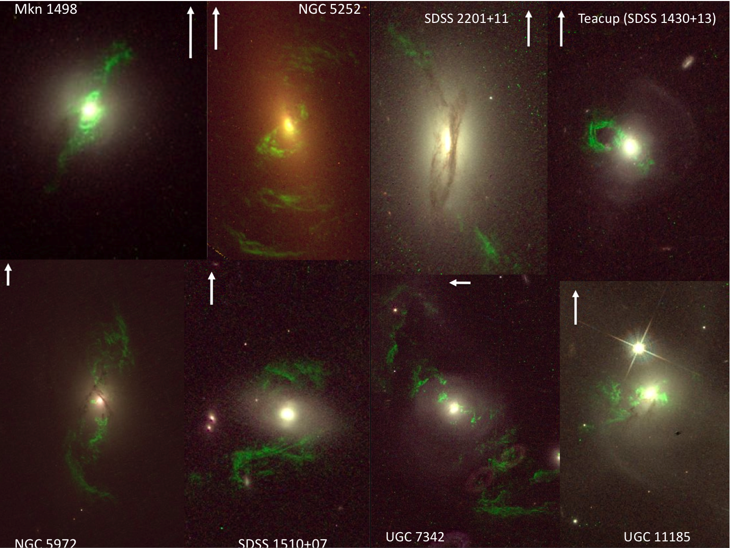
Montage of Hubble images of Voorwerpjes
These are all in interacting galaxies, including merger remnants. This holds as well for possibly all the “parent” sample including AGN which are clearly powerful enough to light up the surrounding gas. Signs include tidal tails of star as well as gas, and dust lanes which are chaotic and twisted. These twists can be modeled one the assumption that they started in the orbital plane of a former (now assimilated) companion galaxy, which gives merger ages around 1.5 billion years for the two galaxies where there are large enough dust lanes to use this approach. In 6 of 8 galaxies we studied, the central bulge is dominant – one is an S0 with large bulge, and only one is a mostly normal barred spiral (with a tidal tail).<?p>

Numerical model of precessing disk of gas from a disrupted companion of NGC 5972
Incorporating spectroscopic information on both internal Doppler shifts and chemical makeup of the gas we can start to distinguish smaller areas affected by outflow from the active nuclei and the larger surrounding regions where the gas is in orderly orbits around the galaxies (as in tidal tails). We have especially powerful synergy by adding complete velocity maps made by Alexei Moiseev using the 6-meter Russian telescope (BTA). In undisturbed tidal tails, the abundances of heavy elements are typically half or less of what we see in the Sun, while in material transported outward from the nuclei, these fractions may be above what the solar reference level. There is a broad match between disturbed motions indicating outward flows and heavy-element fractions. (By “transported” above, I meant “blasted outwards at hundreds of kilometers per second”). Seeing only a minor role for these outflows puts our sample in contrast to the extended gas around some quasars with strong radio sources, which is dominated by gas blasted out at thousands of kilometers per second. We’re seeing either a different process or a different stage in its development (one which we pretty much didn’t know about before following up this set of Galaxy Zoo finds.) We looked for evidence of recent star formation in these galaxies, using both the emission-line data to look for H-alpha emission from such regions and seeking bright star clusters. Unlike Hanny’s Voorwerp, we see only the most marginal evidence that these galaxies in general trigger starbirth with their outflows. Sometimes the Universe plays tricks. One detail we learned from our new spectra and the mid-infared data from NASA’s WISE survey satellite is that giant Voorwerpje UGC 7342 has been photobombed. A galaxy that originally looked as if it night be an interacting companion is in fact a background starburst galaxy, whose infrared emission was blended with that from the AGN in longer-wavelength IR data. So that means the “real” second galaxy has already merged, and the AGN luminosity has dropped more than we first thought. (The background galaxy has in the meantime also been observed by SDSS, and can be found in DR12).

BTA Doppler maps of Voorwerpjes
Now we’re on to polishing the next paper analyzing this rich data set, moving on to what some colleagues find more interesting – what the gas properties are telling us about the last 100,000 years of history of these nuclei, and how their radiation correlates (or indeed anti-correlates) with material being blasted outward into the galaxy from the nucleus. Once again, stay tuned!
Radio Galaxy Zoo searches for Hybrid Morphology Radio galaxies (HyMoRS): #hybrid
First science paper on hybrid morphology radio galaxies found through Radio Galaxy Zoo project has now been submitted!
 In the paper we have revised the definition of the hybrid morphology radio galaxy (HyMoRS or hybrids) class. In general, HyMoRS show different Fanaroff-Riley radio morphology on either side of the active nucleus, that is FRI type on one side and FRII on the other side of their infrared host galaxy. But we found that this wasn’t very precise, and set up a clear definition of these sources, which is:
”To minimise the misclassification of HyMoRS, we attempt to tighten the original morphological classification of radio galaxies in the scope of detailed observational and analytical/numerical studies undertaken in the past 30 years. We consider a radio source to be a HyMoRS only if
(i) it has a well-defined hotspot on one side and a clear FR I type jet on the other, though we note the hotspots may `flicker’, that is their brightness may be rapidly variable (Saxton et al. 2002), and, in the case the radio source has a very prominent core or is highly asymmetric,
(ii) its core prominence does not suggest strong relativistic beaming nor its asymmetric radio structure can be explained by differential light travel time effects. ”
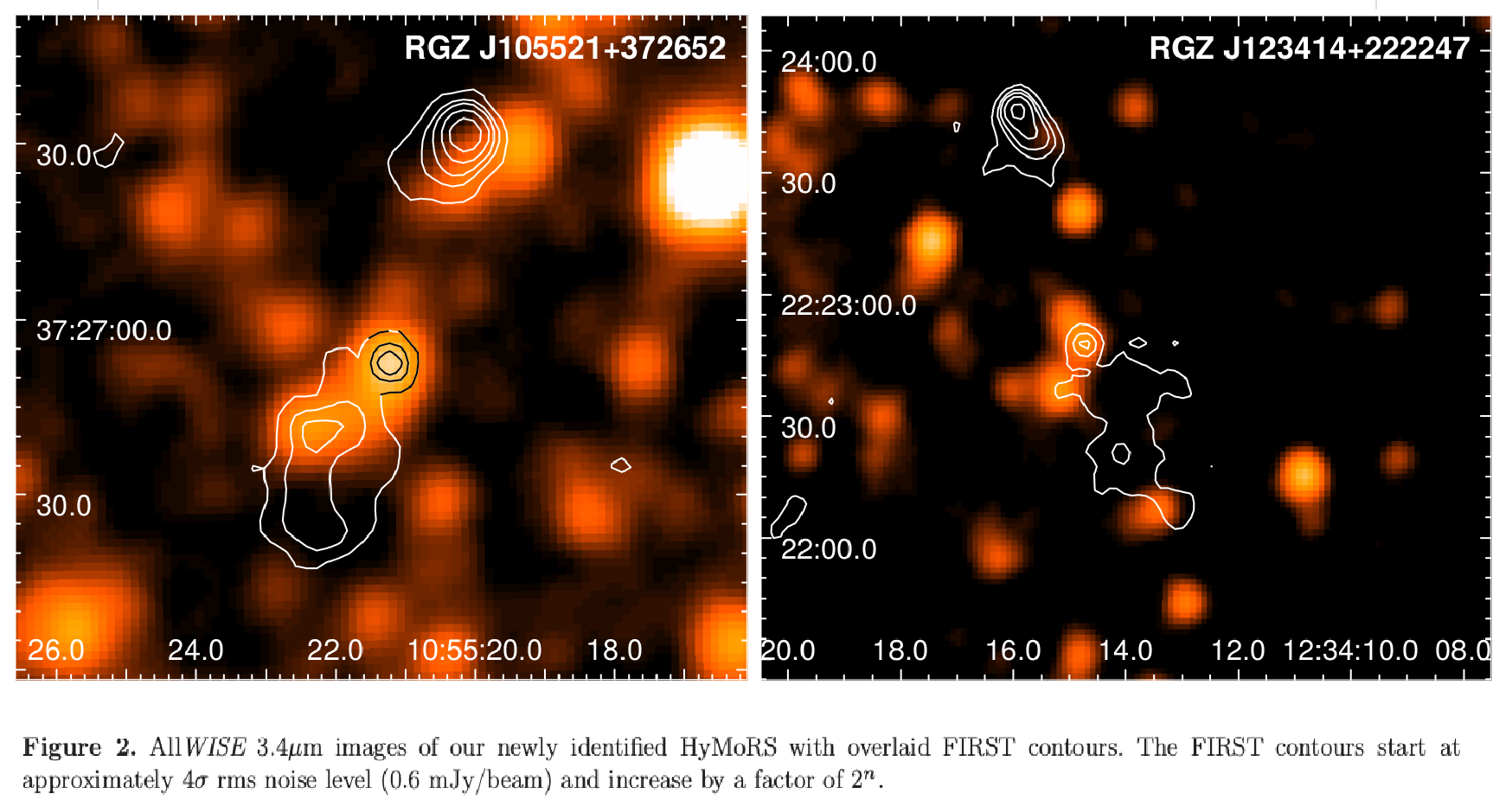
Based on this we revised hybrids reported in scientific literature and found 18 objects that satisfy our criteria. With Radio Galaxy Zoo during the first year of its operation, through our fantastic RadioTalk, you guys now nearly doubled this number finding another 14 hybrids, which we now confirm! Two examples from the paper are below:
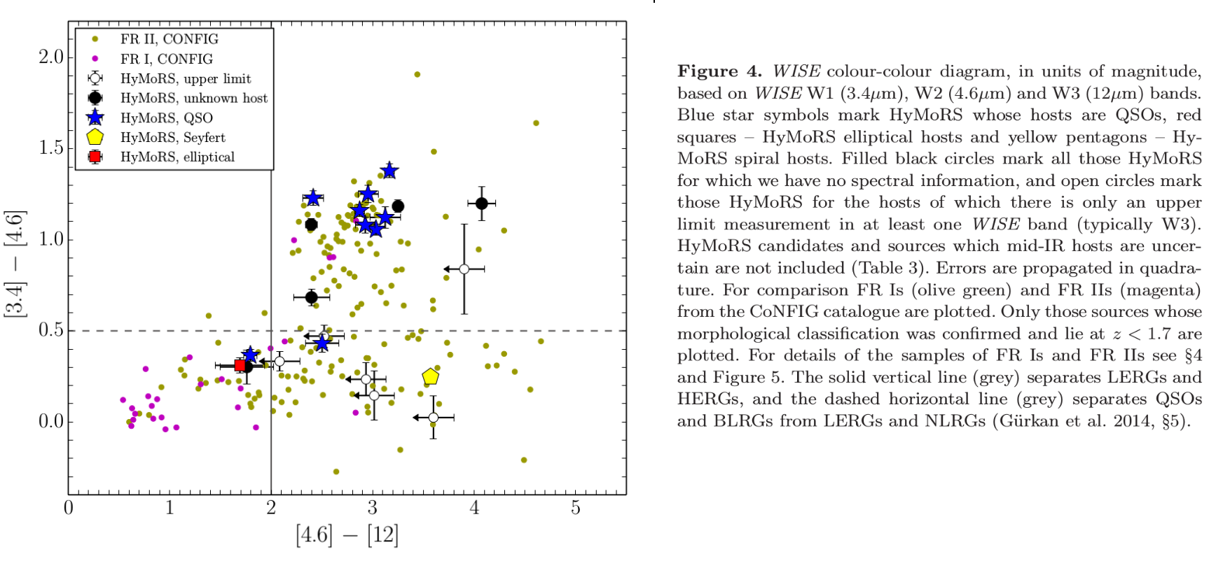
We also looked at the mid-infrared colours of hybrids’ hosts. As explained by Ivy in our last RGZ blog post (https://blog.galaxyzoo.org/2015/03/02/first-radio-galaxy-zoo-paper-has-been-submitted/), the mid-infrared colour space is defined by the WISE filter bands: W1, W2 and W3, corresponding to 3.4, 4.6 and 12 microns, respectively.
The results are below:
For those of you interested in seeing the full paper, we will post a link to freely accessible copy once the paper is accepted by the journal and is in press! 🙂
Fantastic job everyone!
Anna & the RGZ science team
First Radio Galaxy Zoo paper has been submitted!
The project description and early science paper (results from Year 1) for the Radio Galaxy Zoo project has been submitted!

![]() We find that the RGZ citizen scientists are as effective as the science experts at identifying the radio sources and their host galaxies.
We find that the RGZ citizen scientists are as effective as the science experts at identifying the radio sources and their host galaxies.
Based upon our results from 1 year of operation, we find the RGZ host galaxies reside in 3 primary loci of mid-infrared colour space. The mid-infrared colour space is defined by the WISE filter bands: W1, W2 and W3, corresponding to 3.4, 4.6 and 12 microns; respectively.
Approximately 10% of the RGZ sample reside in the mid-IR colour space dominated by elliptical galaxies, which have older stellar populations and are less dusty, hence resulting in bluer (W2-W3) colours. The 2nd locus (where ~15% of RGZ sources are found) lies in the colour space known as the `AGN wedge’, typically associated with X-ray-bright QSOs and Seyferts. And lastly, the largest concentration of RGZ host galaxies (~30%) can be found in the 3rd locus usually associated with luminous infrared galaxies (LIRGs). It should be noted that only a small fraction of LIRGs are associated with late-stage mergers. The remainder of the RGZ host population are distributed along the loci of both star-forming and active galaxies, indicative of radio emission from star-forming galaxies and/or dusty elliptical (non-star-forming) galaxies. See the figure below for a plot of these results.
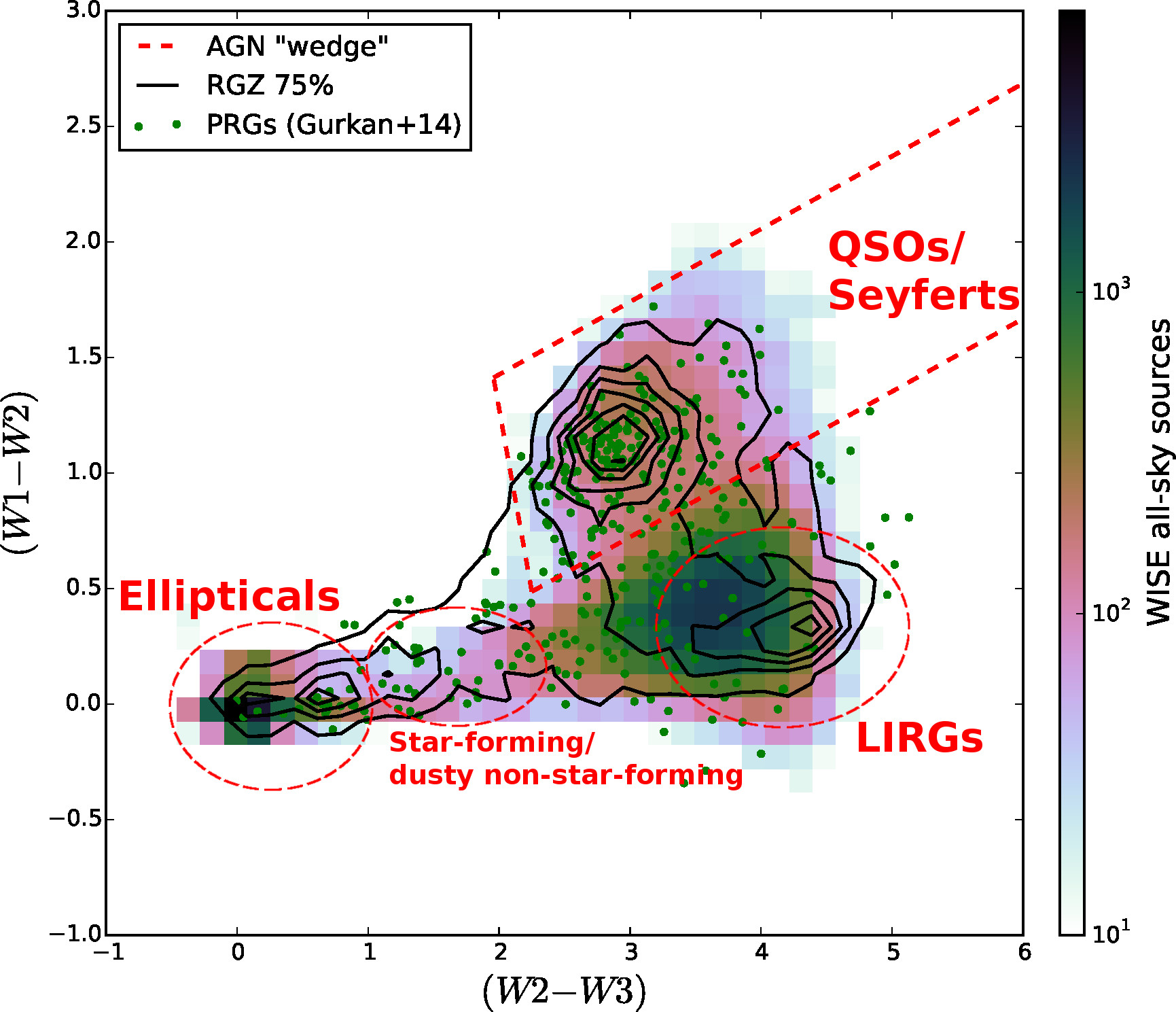 Caption to figure: WISE colour-colour diagram, showing sources from the WISE all-sky catalog (colourmap), 33,127 sources from the 75% RGZ catalog (black contours), and powerful radio galaxies (green points) from (Gürkan et al. 2014). The wedge used to identify IR colours of X-ray-bright AGN from Lacy et al. (2004) & Mateos et al. (2012) is overplotted (red dashes). Only 10% of the WISE all-sky sources have colours in the X-ray bright AGN wedge; this is contrasted with 40% of RGZ and 49% of the Gürkan et al. (2014) radio galaxies. The remaining RGZ sources have WISE colours consistent with distinct populations of elliptical galaxies and LIRGs, with smaller numbers of spiral galaxies and starbursts.
In addition, we will also be submitting our paper on Hybrid Morphology Radio Sources (HyMoRS) in the next few days so stay tuned!
As always, thank you all very much for all your help and support and keep up the awesome work!
Cheers,
Julie, Ivy & the RGZ science team
Zooniverse at Mauna Kea, Day 6: This is the End

Part 1, Part 2, Part 3, Part 4, Part 5
I’m not sure if we’ve been especially unlucky or if this is the norm for observing trips, but we once again the weather is curtailing our telescope time. After a few hours of normal observing, clouds started to blow across the top of Mauna Kea, and now it’s raining outside the dome.
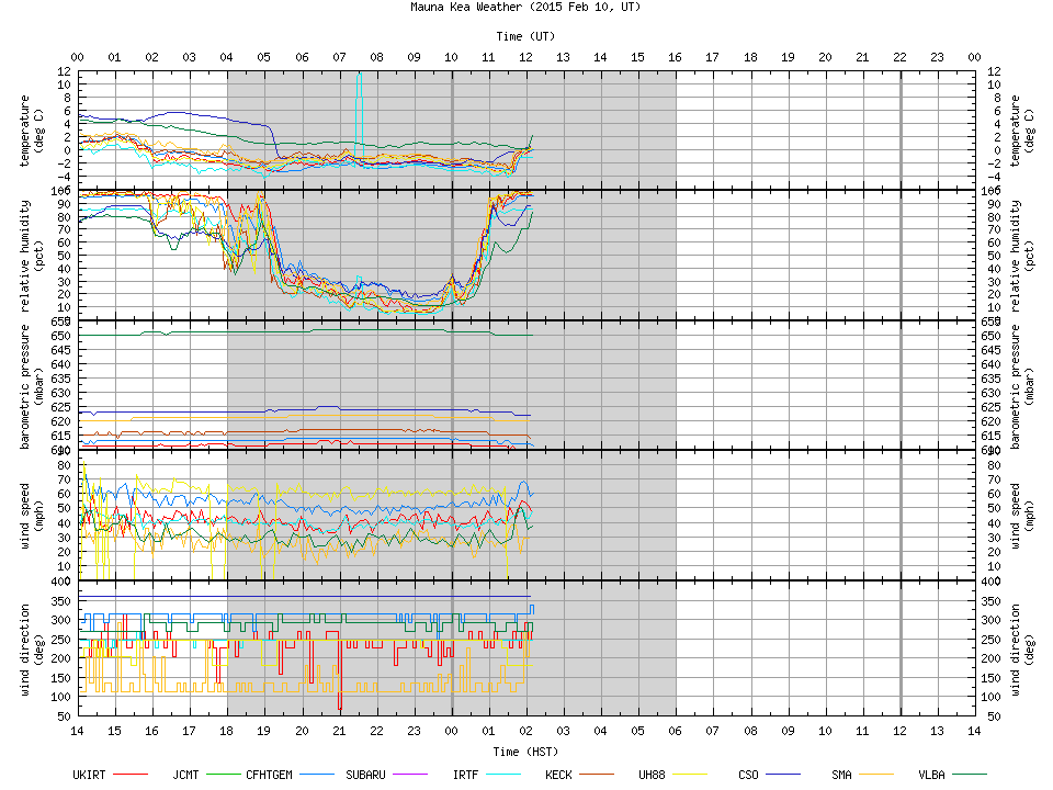
The Dip in the humidity (2nd from the top) represents when we were able to observe.
In the meantime, Becky and I shot a short video tour of the dome a couple days ago you can check out:
Tomorrow, we check out of Hale Pohaku and head down to Hilo for a night. Then I’m off to Chicago and Becky and Sandor are back to Oxford. Even with the bad weather, sleep deprivation, and static electricity, this trip has been a really great experience for me. I now know infinitely more about radio astronomy than I did before! I hope the people doing the real work were able to get all the data they needed.
A Few Notes:
This sums up the general mood
Zooniverse at Mauna Kea, Day 5: The Wind Strikes Back

Part 1, Part 2, Part 3, Part 4
After few good days of observations the wind has returned to ruin our fun. The CSO telescope is supposed to be closed when the wind is above 35mph. Curiously the telescope itself doesn’t have its own anemometer, so we have to rely on readings from the other telescopes on the mountain to decide if it is safe to open the telescope building.
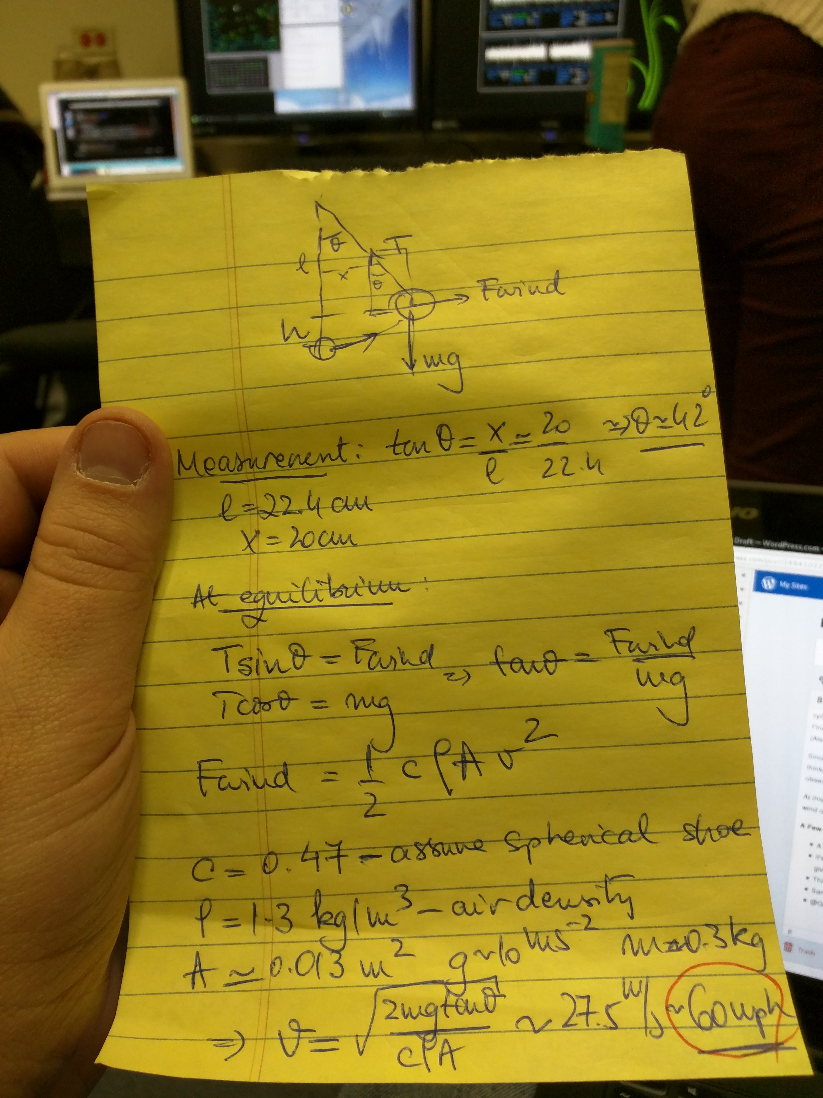
Feeling this entire situation was quite unsatisfactory, I decided to build my own anemometer using a clipboard with a ruler and Becky’s boot, giving you the answer to Chris’s question from earlier tonight:
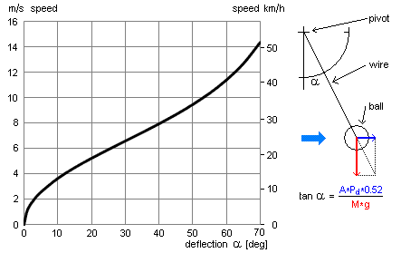
Shout out to Mrs Beck’s AP Physics for me understanding this
Using the above chart we tried to workout the wind speed. We had to do a bit of fudging. We decided the boot was a perfect cylinder (drag coefficient 0.82), and that it weighed about 300g. We also decided not to take into account lower air pressure. Finally when Sandor and I calculated it independently, we got wildly different results, so it was a futile exercise in the end. (Also CSO buy an anemometer)
Sandor doing the hard work!
Since then, we’ve been playing chicken with the wind. Sometimes having to close the dome. Sometimes thinking we can be open, only to have the telescope struggle to stay on target. Sometimes we hear Meg Schwamb‘s wind tracker say “Warning High Winds”. The conditions made us miss out on a second night of observing Comet Lovejoy, and everyone seemed pretty down for most of the night.
Around 1 or 2am the wind finally let up and we were able to start observing, so the night wasn’t a complete loss. Hopefully the weather tomorrow is better.
A Few Notes:
- It’s really hard to get enough sleep. Sleeping at altitude is hard anyway, and adding in trying to sleep during the day gives us all points for degree of difficulty. Everyone has lovely bags around their eyes.
- This is the last day Chris is with us. We’ll be all alone tomorrow night.
- Sandor is succumbing to the static curse now too.
- @GeertHub on Twitter wanted to me to post a screen shot of the telescope software:

- All the Sex & Drugs & Rock & Roll is helping us touch the sky.

Zooniverse at Mauna Kea, Day 4: Stand Back!

Tonight we took a brief break from observing galaxies to train the Caltech Submillimeter Observatory on comet Lovejoy. I was able to help out with the observation in a real life version of:
![Wait, forgot to escape a space. Wheeeeee[taptaptap]eeeeee](https://i0.wp.com/imgs.xkcd.com/comics/regular_expressions.png)
(turns out they have swinging ropes in the control room, who knew?). Sandor and Becky did the actual observing work. Sandor running the telescope, and Becky doing the data reduction to produce a nice graph Chris tweeted:
In the last post, I talked about how the telescope deals with the background noise from the Earth’s atmosphere by ‘chopping’ or alternating reading from its target and a point slightly off the target, then combining the readings to produce a measurement of the target with atmospheric interference removed. This works well for the distant galaxies we are observing, but not with the comet. Chris realized that the comet was too close and large (in a relative sense) for chopping to work. The telescope would take its noise reading while still pointing at the comet.
Instead, we used another, albeit less effective, technique for handling noise. We tuned the telescope to the frequency we were looking for (Carbon Monoxide) took a measurement, and then tuned it to another frequency to measure the background noise. Subtracting the noise measurement from the measurement of our target frequency gives us a clean(-ish) signal.
After that the really exciting bit happened. I got to operate the telescope as we recalibrated it and got ready to point it at our first galaxy of the night. It was pretty easy, telescope operating. Even someone with a BS in Film, like me, can do it. The procedure for moving on our first source was to first pick a bright known object, aim the telescope at it, and have the telescope calibrate its positioning by taking five measurements around the source to figure out the source’s true location.
Once the positioning was calibrated, I ordered the telescope to ‘slew’ (using that new vocabulary) to the galaxy we’re observing, set the exposure time, and then had it ‘chop’. And then ‘chop’ again. And then ‘chop’ again. And again. And you get the idea. I’ve gotten to use a bunch of different cameras, but this was by far the coolest one I’ve operated.

That full-frame Red One is weaksauce next my 10m dish
A Few Notes:
- We ran into to computer glitch around 5 in the morning yesterday. Simon, the telescope manager, kindly helped us fix it.
- “Watts/Hertz or Watts*m^2/Hertz” I overheard Becky saying, triggering deeply repressed memories of doing unit conversion in High School chemistry.
- Sorry there haven’t been as many pictures recently. Stuff inside the control room doesn’t really seem to change that much from night to night.
- There was concern about our comet observation from a collaborator. It turns out the telescope was trying to compensate for the comet’s motion as though it were a distant galaxy, so the above graph still needs a few adjustments applied to it.
- We had some Comet Lovejoy themed music tonight . We didn’t even look at M83.
Zooniverse at Mauna Kea, Day 3: This line is not hidden in the RMS!

It occurred to me I haven’t talked much about the telescope itself. There haven’t been any pictures of it yet either. We’re at the Caltech Submillimeter Observatory which is basically a giant (10m) dish inside a sweet looking disco ball on top of a dormant volcano. It observes at wavelengths somewhere in between infrared and microwave.

The Dish (Astronomers for Scale)
We spend all of our time at the telescope in the control room with everyone hunched over a computer. I’ve learned a couple of the incantations they use to control the telescope. The first command ‘chop’ is what actually makes it record an observation. I wondered why it wasn’t called ‘listen’ or ‘observe’, but it turns out that ‘chop’ pretty accurately describes the motion of the telescope while it records.
The galaxies we’re observing are very distant and faint, and blend in to the background radiation in our atmosphere. To make up for this, the telescope will take a measurement of the source and then another slightly off the source. The controlling computer uses the second measurement to subtract the background noise from its measurement of the source galaxy.
The other command causes the telescope to move. It’s called ‘slew’. When I asked where that name came from, I was given a shrug by the so-called ‘experts’ in the room. So I turned to Google, and found the dictionary definition is to ‘turn or slide violently or uncontrollably in a particular direction’, which sounds like an accurate description of how the telescope’s movement feels from the control room. It’s also originally a nautical term which also feels appropriate.
Observing is serious business. Watching people observe is not!
A few notes from the second half of last evening and this:
- We had a small earthquake! It was exciting. It was shocking. It was only a 3.3! This is the second earthquake Chris, Sandor, and I have experienced and was Becky’s first. Pretty cool.
- Apparently the observations tonight have provided some confusing results. I tried to get Chris to explain what was odd about them. Mostly due to altitude (partly due to working on this), all I could grasp was that they wanted to compare their observations to a nice looking graph with a clear regression line, and the galaxies they are observing are way off in a corner instead of along the line.*
- Becky has a major problem with static electricity.
- Here are some of the songs we’ve been listening to tonight (presented without judgment).
- You can find more pictures of all the other telescopes at the top of Mauna Kea (post about all of them upcoming!) and other photos of the trip here.
* They misinterpreted the data and everything fits now!
Zooniverse at Mauna Kea Day 2: Take that Meteorologists!
(In which dismayed by forecasts of 100mph winds we go to beach and then end up observing anyway)
A brief update on last night, we were actually able to open the telescope in the wee hours of Thursday morning. Sandor and Becky got as far as pointing the telescope and starting to calibrate it when the wind picked back up and forced us to close.
On the bright-side we enjoyed a beautiful sunrise from the top the mountain.
We awoke late in the afternoon, to emails warning us that “Summit Conditions are Extremely Dangerous” and weather predictions of 100mph winds on the top of the mountain. Thinking it would be a lost night, Becky, Sandor, and I took off for Kona, hoping to checkout the ocean and maybe catch the sunset. Chris stayed behind to answer emails.
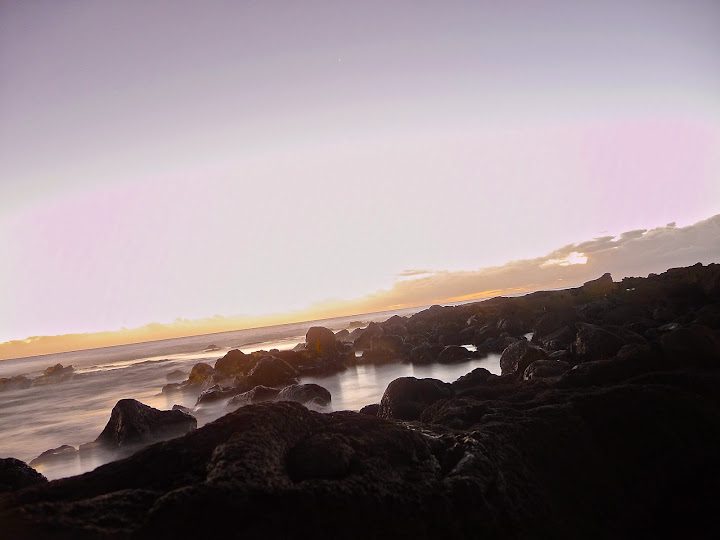
Sooo pretty (Photo by Becky)
It was awesome. Definitely a good decision.
Back at Mauna Kea, the predicted extreme winds never materialized, and Chris and Meg Schwamb were able to open the CSO’s doors for a bit of remote observing, while the beach bums rushed back to Hale Pohaku to join. After a brief wind scare, we made the trip up the mountain to observe on site.

Hard at work! (Photo by Ed)
It turns that radio astronomy is pretty similar to computer programming (my normal Zooniverse occupation), in that it mostly seems to involve typing obscure commands into a shell prompt and then waiting for things to happen. Unlike programming, it also involves stomach churning shifts, as the entire building moves to track the source.
During the waiting periods, I’ve tried to learn more about how the telescope works after being mesmerized by Simon’s, the telescope’s manager, technospeak. One part of the telescope he seemed most eager to show us was the heterodyne receiver. After asking the real astronomers what is was, I was very disappointed to learn that it wasn’t a Terminator weapon. Instead, it’s part of the telescope’s processing pipeline that transforms the signal from the telescope to a frequency where detectors are cheap(er). Anyway it’s certainly a cool looking piece of equipment.
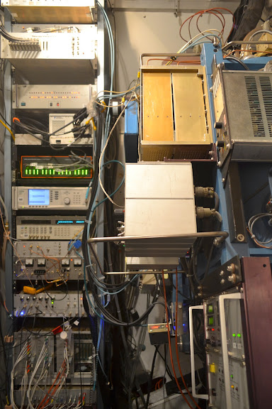
It came form the Future to save the Present (Photo by Sandor)
That’s about it for me tonight. We’ll just be up here listening to some sick jams and looking at distant galaxies. Remember you can find a bunch of pictures of trip (not many of people observing yet though) here.
