
Radio Galaxy Zoo: New tools in Talk
For Zooniverse projects, the science teams have always been really impressed by the users who actively participate in Talk and engage in close inspections and discussions. This is especially true for our newest project, Radio Galaxy Zoo, and the number of excellent questions about larger structure for the powerful radio jets has spurred us to add some new tools to the Talk interface.
The new tools we’ve set up (with the invaluable help of Zooniverse developer Ed) show images of the galaxies and their associated radio jets from other surveys. New images include radio observations from the NRAO VLA Sky Survey (NVSS) and optical images from the Sloan Digital Sky Survey (SDSS). We’ve also included direct links to the FIRST (radio) and WISE (infrared) datasets that we use to make the classification images in the first place.
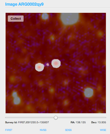
The new tools in RGZ now link to four catalogs (FIRST, NVSS, SDSS, and WISE) for each galaxy along the bottom of each image. FIRST and NVSS are radio surveys, SDSS is optical, and WISE is infrared.
Radio images with wider fields of view, such as NVSS, help to identify structures that may extend beyond the boundaries of the standard RGZ image. These include many of the images being labeled as #overedge in Talk. The NVSS images were taken using the same telescope (the Very Large Array in New Mexico) and at the same wavelength at the FIRST radio images. The main difference is the spacing of the telescopes used to take the observation. NVSS images have a much larger beam size, and are better at resolving large and extended structures. FIRST has a smaller beam size and are more sensitive to compact structures with very accurate positions. FIRST is also about 2.5 times more sensitive than NVSS.
By looking at the NVSS images, both RGZ volunteers and scientists have been able to work together and find potentially new examples of giant radio galaxies in these surveys. Larry Rudnick (@DocR) has started a great discussion on Talk, and we’re still identifying more as the project continues.
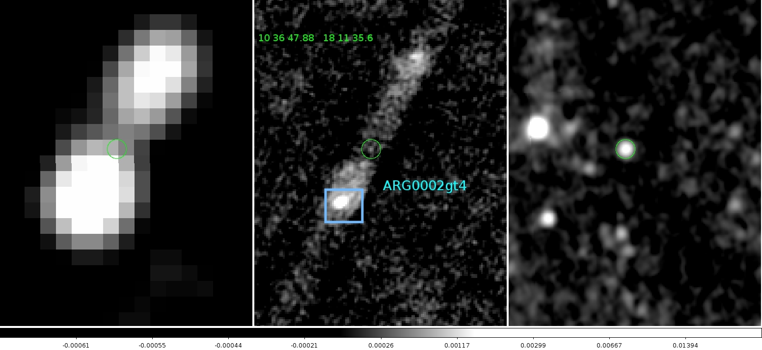
RGZ image ARG0002gt4, as seen in three of the surveys accessible in the new tools. The wide-field radio NVSS image of the jets is on the left; in the middle is the radio FIRST image, showing the better-resolved galaxy core, and on the right is the infrared WISE image showing the host galaxy. Image from Larry Rudnick (UMN).
We’ve also added links to the infrared and optical catalogs that show the galaxies themselves. The infrared images that we show in RGZ come from the WISE spacecraft, an orbiting infrared telescope that carried out an all-sky survey. The new link shows you infrared images of the galaxy in four different infrared bands (3.4, 4.6, 12, and 22 microns), as opposed to the single 3.4 micron image we normally show. Detecting the galaxy at longer wavelengths might mean that it contains more dust than expected, or show whether a feature in one band might be an artifact (not showing up in any of the other bands). We’ve also linked to the optical image from the SDSS; these dusty and distant galaxies are often too faint to show up there, but an optical detection there makes it much more likely that we already have a spectrum for the object.

WISE infrared images of the galaxy ARG0002h6v. Note how the central galaxy shows up strongly in the two bands on the left (3.4 and 4.6 microns), but is not detected in either of the bands on the right (12 and 20 microns).
Let us know if you have suggestions or questions about the new tools; we hope that they’ll continue to lead to many future discoveries with Radio Galaxy Zoo!
Announcing Galaxy Zoo’s machine-learning competition (with prize money!)
Since Galaxy Zoo began in 2007, our scientific results have relied on the classifications of our volunteers. These have always been checked (in small numbers) against expert classifications, and several papers have explored how the Galaxy Zoo data compares to results from computers. Galaxy Zoo has compared well with both expert and automated classifications, and that’s helped underscore the science that your observations have made possible.
While doing real science with the Zooniverse has always been our primary goal, we’re also looking to the future; upcoming telescopes like the SKA, LSST, and just-launched Gaia will have billions of new images and detected objects. This will simply be too large for citizen scientists to handle the full scope of data – even if literally everyone on the planet is involved.
This is where Galaxy Zoo will come in yet again. Our goal, which is shared by many groups of astronomers, is to improve the accuracy of the galaxy classifications that can be performed by computers. We’ve done some of this already (Banerji et al. 2010, Huertas-Company et al. 2011), but it’s still not good enough for much of the science we want to do. If we can make these algorithms better, future datasets for citizen science can be selected in advance; we can automatically process the bulk of the images, but still have citizen scientists play a key role in classifying at the more unusual objects. Citizen scientist results will also provide important calibration for the algorithms, and will continue to look for weird and wonderful discoveries like the Voorwerp.
With that goal in mind, we’re pleased to announce the launch of a data science competition for Galaxy Zoo. We’ve partnered with Kaggle, an online platform for predictive modeling that has a massive amount of experience in similar projects. Also working with us is Winton Capital: they’ve generously agreed to provide prize money for the winners of this competition. The first prize is $10,000 USD — we hope this will help incentivize some really great solutions!
Here’s how the competition works. On the Kaggle website, competitors will be given a large set of JPG galaxy images (taken from Galaxy Zoo 2), as well as a big text file with a few dozen variables for each image. These data are a modified version of the classifications that citizen scientists generated in GZ2 (and published in Willett et al. 2013). The goal for competitors is to come up with an algorithm that will predict what those classifications should be based only on the picture. These algorithms are submitted to Kaggle and tested against a second, private set of GZ2 images and classifications. The highest scores on the new set will win the prize money.

Galaxy Zoo’s machine learning challenge. Hosted by Kaggle and sponsored by Winton Capital.
We’re really excited about this competition. For Winton, this will help them identify promising candidates who are skilled at predictive analysis that they might be interested in hiring. For Galaxy Zoo, we’ll use the results for two major things: efficient selection of sources for upcoming citizen science projects, AND analyzing the results to see how the algorithms relate to physical properties of galaxies.
The competition is open to anyone in the world, and will run for three months, ending on March 21, 2014. Participants will need significant programming experience, and a math/astronomy background would probably help since the project relies on image analysis and machine learning. If you’re interested, check out the project at https://www.kaggle.com/c/galaxy-zoo-the-galaxy-challenge.
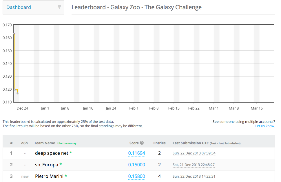
Galaxy Zoo Challenge Leaderboard, as of 22 Dec 2013.
Radio Galaxy Zoo: How were the images made?

Today’s post is from Enno Middelberg, RGZ science team member and astronomer at Ruhr-University Bochum, Germany and expert in interferometry. Enno has kindly agreed to share some details of this complex and highly useful technique for improving the resolution of images.
Radio waves from cosmic objects have been observed since the 1930s, starting with Karl Jansky and Grote Reber. In the beginning, astronomers used single telescopes, some of which looked more or less like TV antennas (and some looked just weird, for example Karl Jansky’s self-made telescope). Whatever the telescope looked like, astronomers understood very well that the resolution of their instruments would never be quite as good as at optical wavelengths. The fundamental reason for this has to do with diffraction theory and Fourier transforms, but the outcome is rather simple: the smallest separation on the sky a telescope can “resolve”, which means, that it can actually tell that there are two things and not one slightly extended thing, is given by the fraction λ/D. Here, λ represents the length of the waves observed (some centimetres in radio astronomy), and D represents the diameter of the telescope (some tens of metres). One can easily calculate that this fraction is of order 0.001-0.004 for a radio telescope, but for an optical telescope the number is much smaller, of order 0.00000005 or so. This means that optical telescopes could separate things on the sky which were much smaller together than the first radio telescopes.
Astronomers had tried to improve on this early on, using something called interferometry. The wavelengths could not be changed (otherwise they wouldn’t be radio telescopes any more, right?), and telescopes could only be made as big as 100m (otherwise they would be too heavy and too expensive). So astronomers took two of the telescopes they had and combined their signals into one. Such a contraption with two telescopes is called an interferometer, and its resolving power is no longer given by the diameter of the dishes, but by their separation. So simply moving the two telescopes further away from one another would increase the resolution – what a fantastic idea! In the 1960s, this technique was much advanced by British astronomer Sir Martin Ryle in Cambridge, and he was awarded the Nobel Prize in Physics for his work in 1974.
In the following decades, Martin Ryle’s innovation was improved upon by astronomers all over the world, creating radio interferometers of various sizes and forms. Radio telescopes sprouted like mushrooms. Ever more powerful telescopes were build: the Very Large Array, theAustralia Telescope Compact Array, the Effelsberg and Greenbank giant single dishes, and many more. Most recently, technical advances have made it possible to build completely digital radio telescopes, such as Lofar. Even though these instruments consist of many more than two radio telescopes, the measurements are always made between any two of them: the Very Large Array, for example, has 27 telescopes, which yields 351 two-telescope inteferometers. Using many more such interferometers improves the image quality and, of course, the sensitivity of the final images.

Radio image with faint emission visible, at the cost of losing details in the bright spots.

Infrared image with radio contours overlayed
Radio images are most commonly reproduced as contour images. This makes them easier to analyse and interpret when printed, and contours are better when very bright and very faint portions of an image have to be shown at the same time. If such information was represented in a grey-scale image, the differences in brightness would not be decipherable. Radio astronomers love contour plots. My wife calls them “fried eggs” and always asks me if the kids can colour them in…
The radio images you’re seeing here are the results of the Australia Telescope Compact Array Large Area Survey (astronomers love acronyms!), or ATLAS for short. Between 2006 and 2009 we have collected data on two small regions in the southern sky to create the basis for an investigation of the way that galaxies evolve. We have used these data to create the radio images you’re seeing when you classify sources. The infrared images were made with the Spitzer telescope, to compare the radio to infrared emission. Radio and infrared waves are not necessarily emitted by the same material and can therefore be displaced from one another in a galaxy. That’s why we need your help to determine what radio blobs belong to which infrared blob!
Radio Galaxy Zoo: a close-up look at one example galaxy
We hope everyone’s been excited about the first few days of Radio Galaxy Zoo; the science and development teams certainly have been. As part of involving you, the volunteers, with the project, I wanted to take the opportunity to examine and discuss just one of the RGZ images in detail. It’s a good way to highlight what we already know about these objects, and the science that your classifications help make possible.
For an example, I’ve chosen the trusty tutorial image, which almost everyone will have seen on their first time using RGZ. We’ll be focusing on the largest components in the center (and skipping over the little one in the bottom left for now).

The tutorial image for Radio Galaxy Zoo
The data in this image comes from two separate telescopes. Let’s look at them individually.
The red and white emission in the background is the infrared image; this comes from Spitzer, an orbiting space telescope from NASA launched in 2003 (and still operating today). The data here used its IRAC camera at its shortest wavelength, which is 3.6 micrometers. As you can see, the image is filled with sources; the round, smallest objects are either stars or galaxies not big enough to be resolved by the telescope. Larger sources, where you can see an extended shape, are usually either big galaxies or star/galaxy overlaps that lie very close together in the sky.
Overlaid on top of that is the data from the radio telescope; this shows up in the faint blue and white colors, as well as the contour lines that encircle the brightest radio components. The telescope used is the Australia Telescope Compact Array (ATCA) in rural New South Wales, Australia. This data was taken as part of the ATLAS survey, which mapped two deep fields of the sky (named ELAIS S1 and CDF-S) in the radio at a wavelength of 20 cm.
So, what do we know about the central sources? From their shape, this looks like what we would call a classic “double lobe” source. There are two radio blobs of similar size, shape, and brightness; almost exactly halfway between them is a bright infrared source. Given its position, it’s a very good candidate as a host galaxy, poised to emit the opposite-facing jets seen in the radio.
This object doesn’t have much of a mention in the published astronomical literature so far. Its formal name in the NASA database is SWIRE4 J003720.35-440735.5 — the name tells us that it was detected as part of the SWIRE survey using Spitzer, and the long string of numbers can be broken up to give us its position on the sky. This is a Southern Hemisphere object, lying in the constellation Phoenix (if anyone’s curious).
The only analysis of this galaxy so far appeared in a paper published by RGZ science team member Enno Middelberg and his collaborators in 2008. They made the first detections of the radio emission from the object, and matched the radio emission to the central infrared source by using an automatic algorithm plus individual verification by the authors. They classified it as a likely AGN based on the shape of the radio lobes, inferring that this meant a jet. It’s also one of the brighter galaxies that they detected in the survey, as you can see below – brighter galaxies are to the right of the arrow. That might mean that it’s a particularly powerful galaxy, but we don’t know that for sure (for reasons I’ll get back to in a bit).
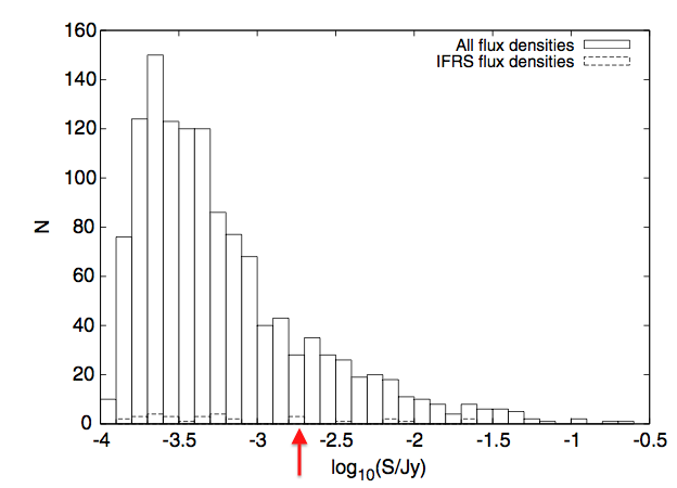
The brightnesses (measured in radio) of galaxies in ATLAS-SWIRE. From Middelberg et al. (2008).
So what we know is somewhat limited – this object has only ever been detected in the radio and near-infrared, and each of those only have two data points. The galaxy is detected at both at 3 and 4 micrometers in the infrared, but the camera didn’t detect it using any of its longer-wavelength channels. This makes it difficult to characterize the emission from the host galaxy; we need more measurements at additional wavelength to determine whether the light we see (in the non radio) is from stars, from dust, or from what we call “non-thermal processes”, driven by black holes and supernovae.
One of the biggest barriers to knowledge, though, is that the galaxy doesn’t currently have a measured distance. Distances are so, so important in astronomy – we spend a massive amount of time trying to accurately figure out how far away things are from the Earth. Knowing the distance tells us what the true brightness of the galaxy is (whether it’s a faint object nearby or a very bright one far away), what the true physical size of the radio jets are, at what age in the Universe it likely formed; a huge amount of science depends critically on this.
Usually distances to galaxies are obtained by taking a spectrum of it with a telescope and then measuring the Doppler shift (redshift) of the lines we detect, caused by the expanding Universe. The obstacle is that spectra are more difficult and more expensive to obtain than images; we can’t do all-sky surveys in the same way we can with just images. This is one reason why these cross-identifications are important; if you can help firmly identify the host galaxy, we can effectively plan future observations on the sources that need it.
Welcome to Radio Galaxy Zoo!
Today’s post is from Ivy Wong, who is delighted to announce our newest Galaxy Zoo project.
Welcome to the extraordinary world of radio astronomy. Observe the Universe through radio goggles and discover the jets that are spewing from the cores of galaxies!
Supermassive black holes lie deep in the cores of many galaxies. And though we cannot directly see these black holes, we do occasionally see the huge jets originating from the cores of some galaxies. However, most of these jets can only be seen in the radio.
 The figure on the left compares the extent of the radio jets from Centaurus A (the nearest radio galaxy to us) to the full moon using the same scale on the sky. Also, the small white dots in this image are not stars but individual background radio sources. The antennas in the foreground are 4 of the 6 antennas that make up the Australia Telescope Compact Array where the radio image was taken.
How do galaxies form these supermassive black holes? And how does having a supermassive black hole affect the evolution of its host galaxy as well as its neighbouring galaxies? Why don’t we see jets in every galaxy with a supermassive black hole? Though much progress has been made in recent years, there are still many open questions such as the above that we can shed light on by amassing a large sample.
To probe the co-evolution of galaxies and their central supermassive black holes, help us map the radio sky by matching the radio jets and filaments to the galaxies (via the infrared images) from whence they came.
 and infrared (red).")
Can you see the infrared galaxy between the radio jets?
This is a matching & recognition problem that humans are still best at, especially in cases where there are radio jets or multiple sources. And it’s an important task, one that will only become more important as the next generation of radio surveys and instruments come online and start producing enormous amounts of data. So if you’re willing to help, please try out the new Radio Galaxy Zoo and help find some growing black holes — and thank you!
We’re Observing at the Very Large Array!
I’m really excited to be able to post that galaxies selected with the help of Galaxy Zoo classifications are being observed at the VLA (Very Large Array) in New Mexico, possibly right now.

It’s the Very Large Array!
The funny thing about observing at the VLA is that you do all of the work for the actual observations in advance.
The VLA runs in queue mode – as an observer you have to submit very (very) detailed information about what you want the telescope to do during your session (called a “scheduling block”) and a set of constraints about when it’s OK to run that (for example you tell them when the galaxy is actually up in the sky above the telescope!). Then the telescope operators pick from the available pool of scheduling blocks at any time to make best use of the array.
This means after you submit the scheduling blocks you just have to sit and wait until you start getting notifications from VLA that your galaxies have been observed. The observing semester for the B-array configuration started on 4th October (had a pause for the US shutdown) and runs until the 13th January 2014. I’m happy to report that we started getting notifications in late November of the first of our 2 hour scheduling blocks having been observed. At the time of writing four of our galaxies have each been observed at least once (we need six repeat visits to each one to get the depth of data we’d like) for a total of 16 hours of VLA time. I’ve been getting notifications every couple of days – which means that as I write this the VLA could be observing one of our galaxies!
Since making these very detailed observation files is the observing prodecure at the VLA – it takes the length of time you’d expect given that…..
So, in September in-between a crazy travel schedule, and with a lot of help from our collaborator Kelley Hess at Cape Town, I spent a lot of time scheduling VLA observations of some very interesting very gas rich and very strongly barred galaxies we identified in the Galaxy Zoo 2 sample (the bit which overlaps with the ALFALFA survey which measures total HI gas in each galaxy).
We have been granted time to observe up to 7 of these fascinating objects (depending on scheduling constraints at the VLA) which I think may reveal some really interesting physics about how bars drive gas around in the discs of galaxies.
You might notice from the picture (and the name) that the VLA is not a “normal telescope”. It’s what astronomers call a radio interferometer. Signals are collected from 27 separate antennas and combined in a computer. This means that as well as observing sources for flux calibration (so we can link how bright our target is through the telescope with physical units) we also have to observe, roughly every 20 minutes or so a “phase calibrator” to be able to know how to correctly add the signals together from each of the antennae (to add them “in phase”).
So a single scheduling block lasting 2 hours for one of our sources comprises:
1. Information to tell the VLA where to slew initially and what instrumentation to use (how to “tune” it to the frequency we know the HI in the galaxy will emit at).
2. A short observation of a known bright source for flux calibration.
Then there’s a loop of
a. Phase calibration
b. Source observation
c. Phase calibration
d. Source observation
and so on – ending with a Phase calibration (on Kelley’s advice we’ll do 5 source observations, and 6 phase calibrations). We have a total of 6 of these blocks for each galaxy, that makes 12 hours of telescope resulting in about 10 hours of collecting 21cm photons per galaxy.
We have to check which times all these sources are visible to the VLA, and set durations for each part which give enough slew time and on source time wherever the sources are on the sky. And this all has to add up exactly to 2 hours to fit the scheduling block.
The benefit of this though is a telescope which acts like it’s much larger than you could ever physically build. We’re trying to detect emission from atomic hydrogen in these galaxies which emits at 21cm. So we need a really large telescope to get a sharp picture.
And just to end, because they’re lovely, here are the four galaxies the VLA has observed so far in the Sloan Digital Sky Survey visible light images.


Thanks again for your help finding these rare and interesting galaxies. They’re rare, because they’re so gas rich and strongly barred – we have previously posted about how we showed strong bars are rare in galaxies with lots of atomic hydrogen. Hopefully we’ll have some exciting results to share once we’ve analysed these data.
(PS. That takes a lot of time too – it’ll be almost 1TB of data to process in total!).
Bars as Drivers of Galactic Evolution
Hello everyone – my name is Becky Smethurst and I’m the latest addition to the Galaxy Zoo team as a graduate student at the University of Oxford. This is my first post (hopefully of many more) on the Galaxy Zoo blog – enjoy!
So far there have been over 100 scientific research papers published which make use of your classifications, some of which have been written by the select few Galaxy Zoo PhD students (most of us are also previous Zooites). The most recently accepted article was written by Edmund, who wrote a blog post earlier this year on how bars affect the evolution of galaxies. As part of the astrobites website, which is a reader’s digest of research papers for undergraduate students, I wrote an article summarising his latest paper. Since the Zooniverse team know how amazing the Galaxy Zoo Citizen Scientists are, we thought we’d repost it here for you lot to read and understand too. You can see the original article on astrobites here, or read on below.
Title: Galaxy Zoo: Observing Secular Evolution Through Bars
Authors: Cheung, E., Athanassoula, E., Masters, K. L., Nichol, R. C., Bosma, A., Bell, E. F., Faber, S. M., Koo, D. C., Lintott, C., Melvin, T., Schawinski, K., Skibba, A., Willett, K.
Affiliation: Department of Astronomy and Astrophysics, University of California, Santa Cruz, CA 95064
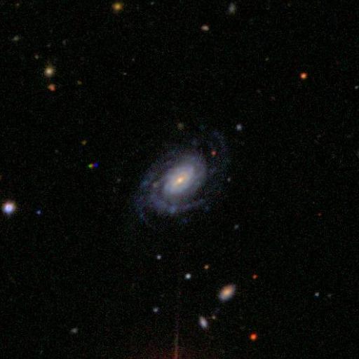
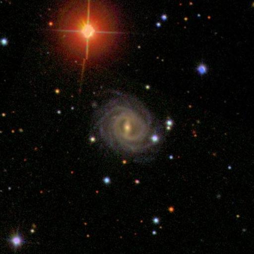
Galactic bars are a phenomenon that were first catalogued by Edwin Hubble in his galaxy classification scheme and are now known to exist in at least two-thirds of disc galaxies in the local Universe (see Figure 1 for an example galaxy).
Throughout the literature, bars have been associated with the existence of spiral arms, rings, pseudobulges, star formation and even Active Galactic Nuclei.

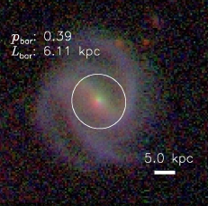
- Figure 1: An example of one of the galaxies inspected in the study by Cheung et al., showing the bar likelihood
and the scaled bar length
.
Bars are a key factor in our understanding of galactic evolution as they are capable of redistributing the angular momentum of the baryons (visible matter: stars, gas, dust etc.) and dark matter in a galaxy. This redistribution allows bars to drive stars and gas into the central regions of galaxies (they act as a funnel, down which material flows to the centre) causing an increase in star formation. All of these processes are commonly known as secular evolution.
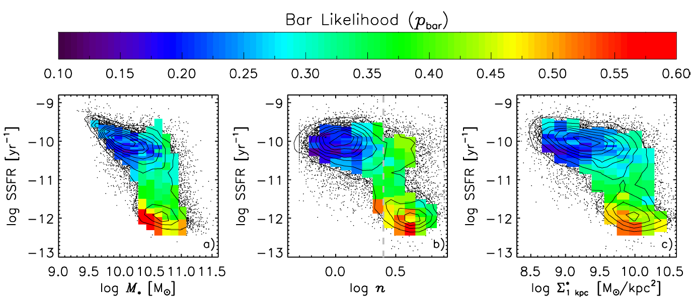
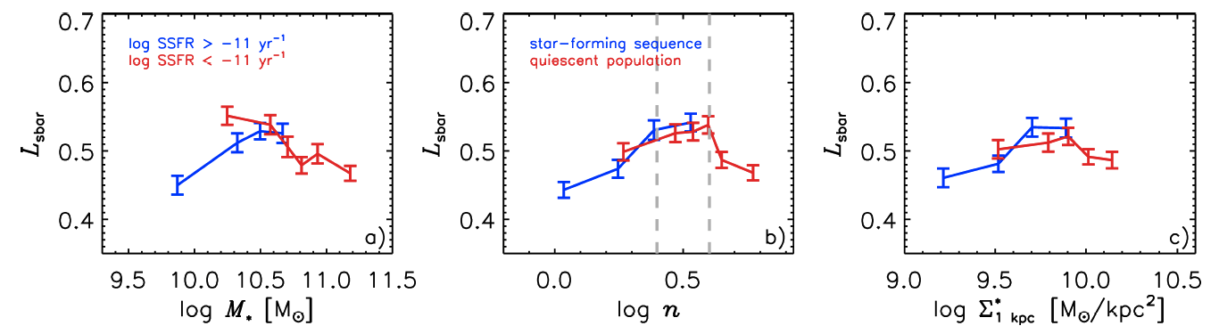
Our understanding of the processes by which bars form and how they consequently affect their host galaxies however, is still limited. In order to tackle this problem, the authors study the behaviour of bars in visually classified disc galaxies by looking at the specific star formation rate (SSFR; the star formation rate as a fraction of the total mass of the galaxy) and the properties of their inner structure. The authors make use of the catalogued data from the Galaxy Zoo 2 project which asks Citizen Scientists to classify galaxies according to their shape and visual properties (more commonly known as morphology). They particularly make use of the parameter
They first plot this bar likelihood using coloured contoured bins, as shown in Figure 2 (Figure 3 in this paper), for the specific star formation rate (SSFR) against the mass of the galaxy, the Sérsic index (a measure of how disc or classical bulge dominated a galaxy is) and the central mass density of a galaxy (how concentrated the bulge of a galaxy is). At first glance, no trend is apparent in Figure 2, however the authors argue that when split into two samples: star forming (log SSFR > -11 

- Figure 2: The average bar likelihood shown with coloured contoured bins for the specific SFR (SFR with respect to the the total mass of the galaxy) against (i) the mass of the galaxy, (ii) the Sérsic index (a measure of whether a galaxy is disc (log n > 0.4) or bulge (log n < 0.4) dominated and (iii) the central surface stellar mass density. This shows an anti-correlation of
Bars become longer over time as they transfer angular momentum from the bar to the outer disc or bulge. In order to determine whether the trends seen in Figure 2 are due to the evolution of the bars or the likelihood of bar formation in a galaxy, the authors also considered how the properties studied above were affected by the length of the bar in a galaxy. They calculate this by defining a property

- Figure 3: The average (in bins of ~ 100 galaxies) length of a galaxy bar (
As before, Figure 3 shows that the trend in the star forming galaxies is for an increase in 
The authors argue that this correlation between
Galaxy drumstick, anyone?
Over the past six years, Galaxy Zoo volunteers have spotted innumerable patterns in the shapes of regular, merging, and fortuitously overlapping galaxies in the various surveys. While we’ve had great success with letters of the alphabet and with animals, searches of both the Forum and Talk haven’t revealed many turkeys so far. In recognition of Thanksgiving in the U.S. this week, we offer this turkey drumstick (or tofurkey, if you’re a veggie like some team members) spotted last year by volunteer egalaxy.

A galaxy (or pair?) at z=0.436, spotted in Galaxy Zoo: Hubble
For those of you who get them, enjoy the break — and let us know what you think about this interesting galaxy (or possible overlapping pair)!
UPDATE: Next Live Hangout: Tuesday, 19th of November, 7 pm GMT

Our next hangout will be next Tuesday at 7 pm European time / 6 pm UK / 3 pm in Chile / 1 pm EST / 10 am PST.
Update: Our next hangout will be next Tuesday at 8 pm European time / 7 pm UK / 4 pm in Chile / 2 pm EST / 11 am PST.
I mention Chile above because two team members will be at a conference in Chile at the time (spreading the word about Galaxy Zoo is a tough job, but someone’s got to do it) and will try to be on the hangout with us.
What do you want us to talk about? We have some ideas but if you have questions, please let us know!
Just before the hangout we’ll update this post with the embedded video, so you can watch it live from here. If you’re watching live and want to jump in on Twitter, please do! we use a term you’ve never heard without explaining it, please feel free to use the Jargon Gong by tweeting us. For example: “@galaxyzoo GONG dark matter halo“.
See you soon!
Galaxy Zoo and undergraduate research: spiral arms, colors, and brightnesses
The guest post below is by Zach Pace, an undergraduate physics student at the University of Buffalo. Zach worked at the University of Minnesota during the summer of 2013 through the NSF’s Research Experience for Undergraduates (REU) program. Zach is continuing to work with Galaxy Zoo data as part of his senior thesis.
Hi, everyone–
My name is Zach Pace. I’m an undergraduate physics student from the University at Buffalo, and I’ve been working on the Galaxy Zoo 2 project at the University of Minnesota since late May with Kyle Willett and Lucy Fortson. My investigation has been twofold: I have been diagramming specific morphological categories in color-magnitude space, and also fitting those data to mathematical functions.
As many readers probably know, a galaxy’s magnitude (overall brightness in the red band, on a log scale) and a galaxy’s color (the difference between the blue magnitude and a red band) are two important quantities for determining what a galaxy might look like (and how it might evolve). Brighter galaxies have more mass (more stars produce more light, of course), and bluer galaxies have a more recent star formation history (this is because young, bright stars tend to be large, bright, and blue). In terms of the whole population, we know, for instance, that elliptical galaxies tend to concentrate in a red sequence, and have typical colors between 2.25 and 2.75. Conversely, the vast majority of spiral galaxies concentrate in a blue cloud between colors 1.25 and 2.0. These two populations are clearly separated in color-magnitude space (this can be seen in the accompanying 2-D histogram, made from Zoo 2 data).

Color-magnitude diagram (CMD) for objects in Galaxy Zoo 2. The lines show fits to the two main populations of elliptical (red) and spiral (blue) galaxies, following the method of Baldry et al. (2004). The green line shows an approximate separation between them.
One of the main goals of Zoo 2 is to gauge the extent to which morphology informs physical characteristics like color and magnitude, so my objective for the summer was to come up with good representations of color and magnitude for all of the smaller sub-populations in Zoo 2.
Several of my results were interesting and surprising. For instance, it has been suggested that spiral galaxies with more arms and spiral galaxies with tighter arm winding (which is to say, a shallower pitch angle) tend to be brighter and bluer. This can be intuitively understood as follows: tighter winding of spiral arms and the presence of more spiral arms indicate, on average, denser gas clouds in those arms, which is tied to increased star formation and bluer color. However, I wasn’t able to measure this in the Zoo 2 data (all the differences were on the order of the histograms’ bin size, about 0.1 magnitude, or about a 10% difference in brightness). This suggests that spiral galaxies, no matter arm multiplicity or winding, are drawn from the same base population.

Color-magnitude diagram (CMD) for spirals in GZ2, split by the number of spiral arms identified in each galaxy. The distribution of colors and magnitudes for galaxies are statistically similar, no matter what the number of spiral arms.
I also came across something unexpected when looking at bulge sizes in face-on disk galaxies. The distribution of galaxies classified by users as bulgeless is starkly different from the distribution of obvious bulge and bulge-dominated galaxies. Furthermore, the population with a bulge that is just noticeable seems to form an intermediate population between the bulgeless and bulge. This observation is also borne out in edge-on disk galaxies: the population of bulgeless edge-on galaxies has a similar shape to the population of face-on galaxies, albeit with stronger reddening on the bright end.

Color-magnitude diagram (CMD) for disk galaxies in Galaxy Zoo 2, split by the relative size of the central bulge. Galaxies that appear to have no central bulge (top) have very different colors and luminosity than those with dominant bulges (bottom).
To fit the distributions, I used a method pioneered about 10 years ago by Ivan Baldry, which fits one parameter after another in our profile functions to find a distribution that converges onto the best fit. It works okay (but not great) for the whole sample, and it fails pretty badly when working with the smaller sub-populations. This is because I have to fit many parameters at once, and do that a bunch of times in a row for the fit to converge, so there are a lot of points of failure. I’m working now at Buffalo towards finding a different and better fitting routine, which will allow us to represent more distributions mathematically.
If you have any questions, feel free to comment below.
