
The Green Valley is a Red Herring
Great news everybody! The latest Galaxy Zoo 1 paper has been accepted by MNRAS and has appeared on astro-ph: http://arxiv.org/abs/1402.4814
In this paper, we take a look at the most crucial event in the life of a galaxy: the end of star formation. We often call this process “quenching” and many astrophysicists have slightly different definitions of quenching. Galaxies are the place where cosmic gas condenses and, if it gets cold and dense enough, turns into stars. The resulting stars are what we really see as traditional optical astronomers.
Not all stars shine the same way though: stars much more massive than our sun are very bright and shine in a blue light as they are very hot. They’re also very short-lived. Lower mass stars take a more leisurely pace and don’t shine as bright (they’re not as hot). This is why star-forming galaxies are blue, and quiescent galaxies (or “quenched” galaxies) are red: once star formation stops, the bluest stars die first and aren’t replaced with new ones, so they leave behind only the longer-lived red stars for us to observe as the galaxy passively evolves.

Example images of galaxies classified by you. There are blue, green and red spirals, and blue, green and red ellipticals.

As @penguin galaxy (aka Alice) put it….
Blue Ellipticals & Red Spirals
The received wisdom in galaxy evolution had been that spirals are blue, and ellipticals are red, meaning that spirals form new stars (or rather: convert gas into stars) and ellipticals do not form new stars (they have no gas to convert to stars). Since you’re taking part in Galaxy Zoo, you know that this isn’t entirely true: there are blue (star-forming) ellipticals and red (passive) spirals. It’s those unusual objects that we started Galaxy Zoo for, and in this paper they help us piece together how, why and when galaxies shut down their star formation. You can already conclude from the fact that blue ellipticals and red spirals exist that there is no one-to-one correlation between a galaxy’s morphology and whether or not it’s forming stars.

The colour-mass diagram of galaxies, split by shape. On the right: all galaxies. On the left: just the ellipticals (or early-types) on top and just the spirals (or late-types) on the bottom. On the x-axis is the galaxy mass. On the y-axis is galaxy colour. Bottom is blue (young stars) and top is red (no young stars).
Blue, Red and…. Green?
A few years back, astronomers noticed that not all galaxies are either blue and star forming or red and dead. There was a smaller population of galaxies in between those two, which they termed the “green valley” (the origin of the term is rather interesting and we talk about it in this Google+ hangout). So how do these “green” galaxies fit in? The natural conclusion was that these “in between” galaxies are the ones who are in the process of shutting down their star formation. They’re the galaxies which are in the process of quenching. Their star formation rate is dropping, which is why they have fewer and fewer young blue stars. With time, star formation should cease entirely and galaxies would become red and dead.
The Green Valley is a Red Herring
Ok, why is this green valley a red herring you ask? Simple: the green valley galaxies aren’t a single population of similar galaxies, but rather two completely different populations doing completely different things! And what’s the biggest evidence that this is the case? Some of them are “green spirals” and others are “green ellipticals”! (Ok, you probably saw that coming from a mile away).
So, we have both green spirals and green ellipticals. First: how do we know they must be doing very different things? If you look at the colour-mass diagram of only spirals and only ellipticals, we start to get some hints. Most ellipticals are red. A small number are blue, and a small number are green. If the blue ellipticals turn green and then red, they must do so quickly, or there would be far more green ellipticals. There would be a traffic jam in the green valley. So we suspect that quenching – the end of star formation – in ellipticals happens quickly.
In the case of spirals, we see lots of blue ones, quite a few green one and then red ones (Karen Masters has written several important Galaxy Zoo papers about these red spirals). If spirals slowly turn red, you’d expect them to start bunching up in the middle: the green “valley” which is revealed to be no such thing amongst spirals.

We can time how fast a galaxy quenches. On the x-axis is the optical colour, dominated by young-ish stars, while on the y-axis is a UV colour, dominated by the youngest, most short-lived stars.
Galaxy Quenching time scales
We can confirm this difference in quenching time scales by looking at the ultraviolet and optical colours of spirals and ellipticals in the green valley. What we see is that spirals start becoming redder in optical colours as their star formation rate goes down, but they are still blue in the ultraviolet. Why? Because they are still forming at least some baby stars and they are extremely bright and so blue that they emit a LOT of ultraviolet light. So even as the overall population of young stars declines, the galaxy is still blue in the UV.
Ellipticals, on the other hand, are much redder in the UV. This is because their star formation rate isn’t dropping slowly over time like the spirals, but rather goes to zero in a very short time. So, as the stellar populations age and become redder, NO new baby stars are added and the UV colour goes red.
It’s all about gas
Galaxies form stars because they have gas. This gas comes in from their cosmological surroundings, cools down into a disk and then turns into stars. Galaxies thus have a cosmological supply and a reservoir of gas (the disk). We also know observationally that gas turns into stars according to a specific recipe, the Schmidt-Kennicutt law. Basically that law says that in any dynamical time (the characteristic time scale of the gas disk), a small fraction (around 2%) of that gas turns into stars. Star formation is a rather inefficient process. With this in mind, we can explain the behaviour of ellipticals and spirals in terms of what happens to their gas.

A cartoon version of our picture of how spiral galaxies shut down their star formation.
Spirals are like Zombies
Spirals quench their star formation slowly over maybe a billion years or more. This can be explained by simply shutting off the cosmological supply of gas. The spiral is still left with its gas reservoir in the disk to form stars with. As time goes on, more and more of the gas is used up, and the star formation rate drops. Eventually, almost no gas is left and the originally blue spiral bursting with blue young stars has fewer and fewer young stars and so turns green and eventually red. That means spirals are a bit like zombies. Something shuts off their supply of gas. They’re already dead. But they have their gas reservoir, so they keep moving, moving not knowing that they’re already doomed.

A cartoon version of how we think ellipticals shut down their star formation.
Ellipticals life fast, die young
The ellipticals on the other hand quench their star formation really fast. That means it’s not enough to just shut off the gas supply, you also have to remove the gas reservoir in the galaxy. How do you do that? We’re not really sure, but it’s suspicious that most blue ellipticals look like they recently experienced a major galaxy merger. There are also hints that their black holes are feeding, so it’s possible an energetic outburst from their central black holes heated and ejected their gas reservoir in a short episode. But we don’t know for sure…
So that’s the general summary for the paper. Got questions? Ping me on twitter at @kevinschawinski
The Curious Lives of Radio Galaxies – Part Two
This is the second half of a description of radio galaxies from Anna Kapinska, Radio Galaxy Zoo science team member.
Last time we discussed the early and mid stages of radio galaxy life that take up the majority of the radio galaxy lifetime. Today we will go much further following paths of aging radio galaxies.
‘Only few of us get here’
As we discussed last time, radio galaxies are typically between tens and hundreds of kilo- parsecs in size (30 thousands – 3 million light-years). However, some of our buddies will grow to enormous sizes. Once a radio galaxy reaches one Mega-parsec in size (3.3 million light-years across) it’s called a giant – that is, a giant radio galaxy. Not every radio galaxy will reach such enormous sizes; only the most powerful ones whose environments are not extremely dense do. We don’t see too many giant radio galaxies. There are two main problems. One is that they are of low radio luminosity, and so our telescopes are not always sensitive enough to detect more than a subset of radio galaxies reaching this stage of their lives. The other problem is that giants are often composed of numerous bright knots spread over a large area and it’s difficult for us to tell which of these knots are associated with the giant and which are from unrelated sources.

Figure 5: 3C 236, the second largest giant radio galaxy, extends nearly 15 million light- years across. It is located at a redshift z = 1.0 and has angular dimensions of over 40 arc-minutes in radio images. Credits: NVSS, WRST, Mack et al. 1996.
Giant radio galaxies are usually hundred of thousands, or more, years old and they are very large and extended. They can tell us a lot about what is going on within the space in between galaxies in groups and clusters, and that’s why radio astronomers cherish these giants! The largest giant radio galaxy known is 4.5 Mega-parsecs across (named J1420-0545), which is almost 15 million light-years! In radio images these radio galaxies extended over 20 or 30 arc-minutes, which means you will normally see only one of their lobes at a time in any of the Radio Galaxy Zoo images we classify. This is also the reason why we would tag these Radio Galaxy Zoo images as #overedge or #giants.
Fading away
But radio galaxies will not grow to infinity, they will eventually die. What happens then is that the radio galaxy starts fading away. Physically, at this point, the supermassive black hole stops providing jets with fresh particles, which means the jets and lobes or radio galaxy are not fed with new material. The electrons in the radio galaxy lobes have a finite amount of energy they can release as light, and so the lobes simply fade away until they are no longer visible with our telescopes. Dying radio galaxies become progressively less powerful, and less pronounced: no bright jet knots nor hotspots are present within the lobes anymore (see Figure 6). Eventually we can’t see these radio galaxies any more with our telescopes. You would typically mark these radio sources as #relics or #extended in Radio Galaxy Zoo images. It takes only ten thousand years for the brightest features of radio galaxy lobes to disappear, which is barely 0.01% of the total lifespan of radio galaxy. Again, just as the birth, it’s a blink of an eye!
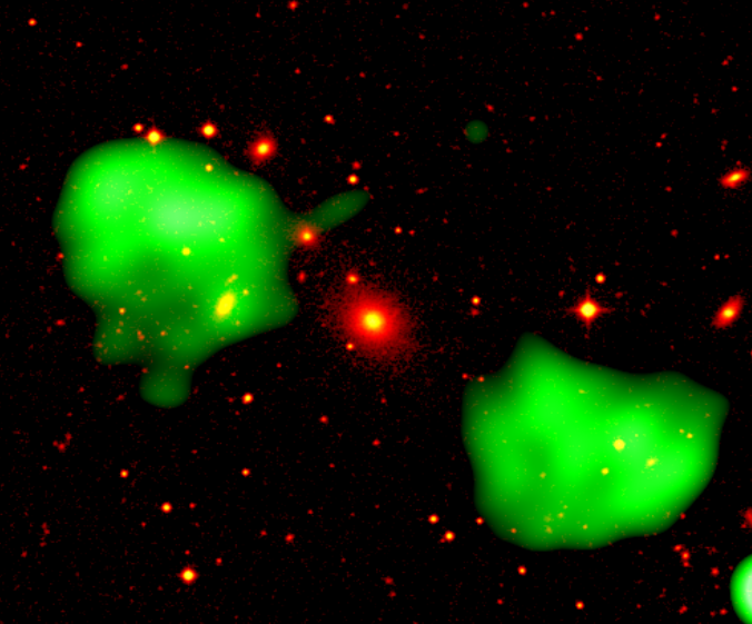
Figure 6: A prototypical dead (relic) radio galaxy, B2 0924+30. Radio waves are imaged in green, while optical image from SDSS is in yellow-red. The angular dimension of this galaxy is 13.5 arc-minutes, and it lies at a redshift z = 0.027, what translates to 430 kilo-parsec (1.4 million light-years) in size. Credits: Murgia
Rebirth
So is that the end?
Well… not really! Astronomers have seen evidence that radio galaxies re-start. What does that mean? That means radio galaxies sort of resurrect. After switching off, the supermassive black hole is radio silent for a while, but it can become active again; that is the whole cycle of radio galaxy life can start all over again. A single host galaxy can have multiple radio galaxy events. We still don’t know the ratio of how long the galaxy is in quiet, silent stage, to how long is in its active, violent radio galaxy forming stage. We also do not know if all galaxies go through the active, radio galaxy forming stage, or whether it’s just some of them. And we don’t know what exactly is the process that makes the galaxies switch on and off. But details on that… that’s yet another story!

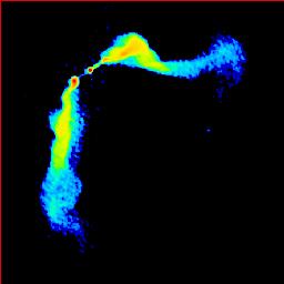
Figure 7: Re-started radio galaxy, PKS B1545-321. This radio galaxy has the so-called double-double structure, which consists of two pairs of double lobes. The outer pair of lobes are older and they are slowly fading away. The inner pair of lobes are created after the radio galaxy is born again. This radio galaxy is also a giant, the outer lobes extend to one Mega-parsec (3 million light-years). Credits: Safouris et al 2002.
The Curious Lives Of Radio Galaxies – Part One
Today’s blog post is written by Radio Galaxy Zoo science team member Anna Kapinska, who works on radio jets and studies how they affect the galaxies which host them at various stages of the Universe’s evolution. This is the first of a two-part series.
As most of you know by now (after classifying hundreds of radio and infrared images in our amazing Radio Galaxy Zoo!) radio galaxies are not the type of object that most of us are used to. There’s no stars and dust; no light from that. It’s all about the jets – outflows of particles ejected from the vicinity of the galaxy’s monstrous supermassive black hole and moving nearly at the speed of light. Some of these particles, electrons, emit light while spiralling in the black hole magnetic field. By no means are the radio galaxies stationary or boring!

Figure 1: The famous Hercules A radio galaxy. The radio emission is imaged in pink and is superimposed on optical image (black/white) of the field. You can clearly see the jets extending from the central host galaxy to feed the lobes. Credits: VLA.
Radio galaxies can live for as long as a few hundred thousand or even a few million years. They grow and mature over that time, and so they change. They even don’t disappear straight after they die; that takes time too. So, how does the life of a radio galaxy look like?
Just as for ourselves, humans, we have names for different stages of radio galaxy life. There are newborn and young radio galaxies. There are adults – these are the most often encountered individua. There are also old, large giants. And there are dead radio galaxies – the slowly fading away breaths of magnificent lives – a rare encounter as they don’t stay with us for too long. So, how do these radio galaxies look like and what exactly happens during their lives? Over the next two blogs I will take you through the evolutionary stages of radio galaxies.
Let’s start off with a simple plot astronomers like to use for an overview of a radio galaxy evolution during its lifetime. The plot describes how the radio luminosity changes with the radio galaxy size (Figure 2). The larger the radio galaxy, the older it is (usually), so we can trace the changes in radio galaxy luminosity and structure (size) as it gets older.
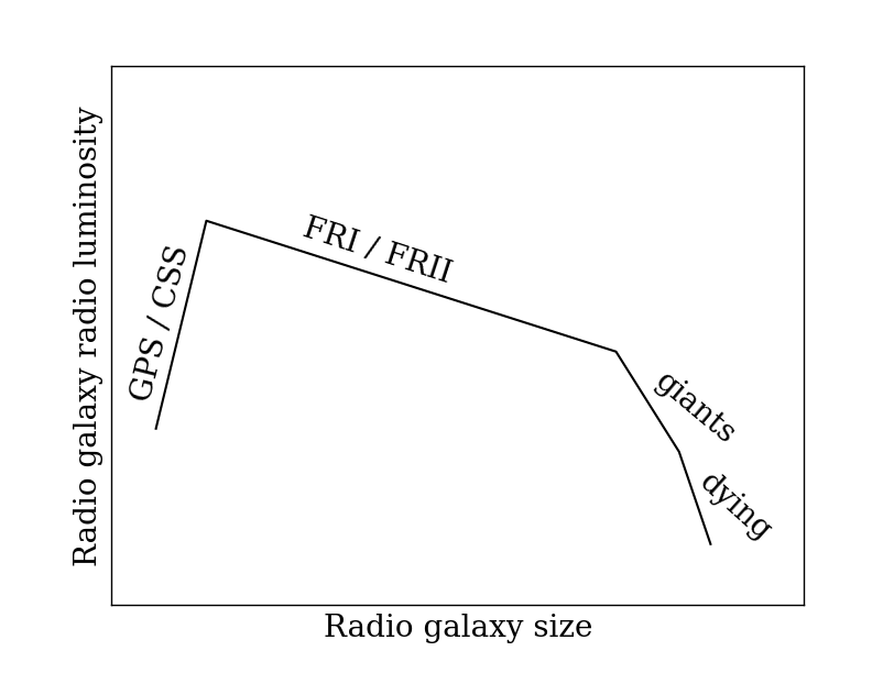
Figure 2: A schematic view of different stages of a radio galaxy life. Credit: Kapinska.
The early years
After a radio galaxy is born it will be growing up very quickly – in a blink of an eye its jets will be penetrating dense environments out to the borders of the host galaxy (the one you can see in optical and infrared wavelengths). Astronomers call these sources GPS (Gigahertz peaked sources) and CSS (compact steep spectrum) radio sources. The GPS/CSS sources are very small; they reach only kilo-parsec distances from the central black hole (3.5 thousand light years), which is merely few arc seconds, or even less, in radio images. This is the reason why we usually detect them as compact radio sources; however, one can sometimes see their double radio structure (that is the jets) in very high resolution radio images (Figure 3), hence really they are just mini-doubles!

Figure 3: A typical CSS radio source, 3C 237, as seen with the FIRST survey (left) and with 20 times higher resolution VLA observations (right). This small radio galaxy lies at a redshift z = 0.877 and is only 9 kilo-parsecs (30 thousand light years) in size. Credits: FIRST, Akujor & Garrington 1995.
This stage of radio galaxy life is the only one at which the radio galaxy luminosity rises steeply as the source grows in size. The stage lasts only for tens to hundreds of thousands of years, which is barely 0.1% of the radio galaxy’s lifetime. This means there is a very short window of time when we can spot CSS and GPS sources, but there are many of these sources around and they are also very bright (their radio luminosities are typically the maximum a radio galaxy can reach) so we often detect them.
The adulthood
After the childhood radio galaxies enter the adulthood. Astronomers have dozen of names to describe the adult radio galaxies and this depends on their structure observed in radio waves, but really, what these radio galaxies have in common is their age and size. They are usually tens to hundreds of millions of years old, and between tens and hundreds of kilo-parsecs in size (30 thousands – 3 million light-years). The luminosity of these radio galaxies slowly drops as they penetrate through the intergalactic space. When you inspect the Radio Galaxy Zoo images, these radio sources are the #hourglass, #doublelobe and #plumes. 3C 237 and Centaurus A are fantastic examples of what we usually see! (Figure 4).
You will quickly notice that there are two main types of these radio galaxies; one type that has very strong radio emission at the end of the lobes (#hourglass, #doublelobes) which is the signature of jets pushing through the ambient medium around radio galaxy. These radio galaxies are called FR IIs by radio astronomers, and the bright spots at the ends of the lobes are called hotspots. The second type has their maximum radio luminosity close to the supermassive black hole or half way through the lobes; these are #plumes within the Radio Zoo and are tagged FRIs by radio astronomers. Plumes are less powerful than the hourglass, but they are even more of a challenge to astronomers!

Figure 4: The FRII type 3C 237 radio galaxy (left) is 290 kilo-parsecs (0.95 million light-years) across. You can clearly see the bright yellow spots at the end of the radio lobes (orange). The blue objects are the optical galaxies and stars, and the white central object is the host galaxy of 3C 237. On the right is huge FR I type Centaurus A radio galaxy which is 700 kilo-parsecs (2.3 million light-years) in size; its radio structure in this image is marked in violet and in the centre we can see optical image of its host galaxy. In the left bottom insert of the image you can see the zoom-in of Centaurus A host galaxy together with small scale jets feeding the larger radio structure. Credits: NRAO, CSIRO/ATNF, ATCA, ASTRON, Parkes, MPIfR, ESO/WFI/AAO (UKST), MPIfR/ESO/APEX, NASA/CXC/CfA
The radio galaxy adult stage will be the majority of their lifetime, and that’s why they are the radio galaxies and radio structures one would typically see. Next time we will see what happens when the radio galaxy gets old!
Reflections on Voorwerpjes

We’re in the middle of an observing run at the Lick 3m Shane telescope, with the first part devoted to polarization measurements of the Voorwerpje clouds (which is to say, giant clouds of ionized gas around active galactic nuclei found in the Galaxy Zoo serendipitous and targeted searches), and just now switching to measure spectra to examine a few new candidate Voorwerpjes, and further AGN/companion systems that may shed light on similar issues of how long AGN episodes last.

Polarization measurements can be pretty abstruse, but can also provide unique information. In particular, when light is scattered, its spectra lines are preserved with high fidelity, but light whose direction of polarization (direction of oscillation of its electric field when considered as a wave) is perpendicular to the angle it makes during this operation is more likely to reach us instead of being absorbed. This is why polarized sunglasses are so useful – glare from such scattering light can be reduced by appropriate orientation of the polarizing filter.
In our context, polarization measurements tell us something about how much of the light we see is secondhand emission from the AGN rather than produced on the spot in the clouds (admittedly as a side effect of the intense UV radiation from the nucleus), and will show us whether we’re fortunate enough that there might be a dust cloud reflecting so much light that we could look there to measure the spectrum of the nucleus when it was a full-fledged quasar. (This trick has worked for supernovae in our galaxy, which is how we know just what kind of supernova was seen in 1572 despite not having spectrographs yet).
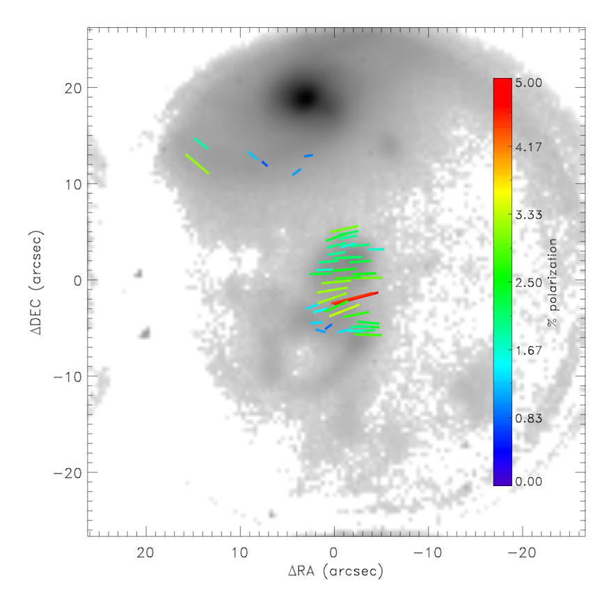
Polarization wizard Sebastian Hoenig (now at the Dark Cosmology Center in Copenhagen) has already produced preliminary calibrations and maps from these new data. Here are some visualizations. In each case, the lines show the direction of polarization. Their length and color show the fraction of light which is polarized at points where there is enough to measure. This fractional polarization tells about the mix of light arising on the spot (even if secondhand due to UV radiation ionizing the gas) and that reflected from dust particles. There is a telltale annular or bull’s-eye pattern when the scattered light originates in a central source, which we see over and over (as if we hadn’t figured out to blame the galaxy nuclei anyway).
First up is a personal favorite, UGC 7342 (the last one to have its Hubble images obtained, and among the largest and brightest of the Galaxy Zoo sample).

The next one, Markarian 78, is less familiar, oddly because it makes perfect sense (so it has not figured much in the followup observations). In this case, we see a bright and obvious active nucleus, one which is powerful enough to light up the giant gas clouds without having changed over the past 60,000 years or so.

For comparison, here is a polarization map of IC 2497 and Hanny’s Voorwerp itself, from data obtained last year (the first time the weather let us get useful results). Sometimes we can hear the Universe laughing – a quick simulation shows that the reflected light from the nucleus, when it was a quasar, is just a bit too faint for us to have seen its signature broad emission lines in any of the Voorwerp spectra.
As we switch into measuring spectra for the next few nights, the aim changes to a combination of looking at a few new Voorwerpje candidates from the Galaxy Zoo forom, and a set of newly-identified AGN/galaxy pairs which may let us study the same issues of AGN lifetimes. We can sort of settle into a routine – Anna Pancoast does calibrations and setup during the day and hands over to Vardha Bennert to finish observations during the night. I typically get to work before Vardha finishes the last galaxy observation (thanks to the time-zone difference) and transfer data to start analysis, so we can change the next night’s priorities if something interesting shows up. It takes a (global) vllage, but then if there’s been any single meta-lesson from Galaxy Zoo, that would be it.
IFRS: The first supermassive black holes?
Today’s Radio Galaxy Zoo post is by Ray Norris, our Project Advisor. Ray researches how galaxies formed and evolved after the Big Bang, using radio, infrared, and optical telescopes.
In Radio Galaxy Zoo, some bright radio sources don’t have any infrared sources at all associated with them, and they have been given the hashtag #ifrs, for Infrared-Faint Radio Sources. So what are these IFRS?
In 2006, we discovered about 1000 radio sources in the Australia Telescope Large Area Survey (ATLAS). Conventional wisdom told us that all of these would be visible in the infrared observations taken by the Spitzer Space Telescope, as part of the SWIRE project. So we were astonished to find that about 50 of our sources were not listed in the SWIRE catalog. Could they be bugs in our data? After eliminating iffy sources, we were left with 11 sources that are bright in the radio but invisible in the infrared images. We dubbed these objects Infrared-Faint Radio Source (IFRS). With hindsight, we should have thought of a better name for them. But at the time we didn’t know that they would turn out to be important!

A very deep infrared image (from this paper), made by stacking images from the Spitzer Space Telescope at the positions of IFRS (shown by the cross-hairs). This image, about 300 times deeper than the WISE images currently being used in Radio Galaxy Zoo, shows that not only is there no infrared counterpart at WISE levels, but even if you go enormously deeper, there’s still almost nothing there in the infrared.
We suggested in 2006 that these might be high-redshift active galaxies – galaxies whose emission is dominated by a super-massive black hole at their centre (the galaxies you are looking at in Radio Galaxy Zoo). This was surprising, because we were finding so many of them that it meant there must be far more supermassive black holes in the early Universe than found by deep optical surveys, such as SDSS (whose images we use in Galaxy Zoo). It’s also far more than can be accounted for by conventional hierarchical models of super-massive black hole formation. Naturally, our colleagues were sceptical, and most of us harboured our private doubts too. But over the next few years we tested this idea and its alternatives. Gradually our confidence grew that these were indeed high-redshift active galaxies.
In 2011 we showed that they were similar to high-redshift radio galaxies (HzRG) but even more extreme. Crucially, we suggested that they follow the same correlations between the radio and infrared emission as the HzRG. If this suggestion turned out to be correct, then that would push them to be amongst the first supermassive black holes in the Universe.
Fortunately, it was possible to test this hypothesis by measuring the redshifts of less extreme objects, to see if they followed these same correlations. Two new papers confirm that they do indeed follow this correlation. In one, Andreas Herzog and his colleagues use the European Very Large Telescope to measure the redshifts of three of these less extreme objects, and find they lie on the correlation, at redshifts between 2 and 3, just as predicted. In the other paper Jordan Collier and his colleagues take exactly the same data now being shown in Radio Galaxy Zoo, and search for objects which are relatively much brighter in the FIRST (radio) data than in the WISE (infrared) data. 1,317 of these are found, of which 19 have measured redshifts. Again, all but one of these lie in the redshift range 2 to 3. This is strong support for the hypothesis!
Armed with this, we are increasingly confident that the most extreme IFRSs that will turn up in the fainter ATLAS and COSMOS field, to be released in Radio Galaxy Zoo in a few weeks, will include many supermassive black holes formed in the first half-billion years after the Big Bang. According to conventional hierarchical black hole formation models, these shouldn’t exist. So the race will be on to identify them and measure their redshifts using instruments like ALMA.
Not everything in Radio Galaxy Zoo classified as being an IFRS will turn out to be a high-redshift black hole, as the data currently being displayed (FIRST and WISE) are not deep enough to pick out the really high-redshift objects. But when the new ATLAS data are loaded into RGZ in a few weeks, almost every object that appears in the radio but not in the infrared will be one of these enigmatic objects. We can’t wait to see how many you find!
How do black holes form jets?

This post was written by Radio Galaxy Zoo team member Stas Shabala, an astronomer at the University of Tasmania.
The supermassive black holes at the hearts of galaxies are supposed to be simple. For someone looking at a black hole from afar, physicists tell us all black holes can be described by just three parameters: their mass, electric charge, and spin. For really big black holes, such as the ones astronomers deal with, things are even simpler: there is no charge (that’s because they are so big that there would always be enough neighbouring positive and negative charges to more or less cancel out). So if you know how heavy a black hole is, and how fast it spins, in theory at least you have enough information to predict a black hole’s behaviour.
Of course the black holes in Radio Galaxy Zoo often have at least one other, quite spectacular, feature – bright jets of radio plasma shooting through their host galaxy and into intergalactic space. Where do these jets come from?, I hear you ask. This is a very good question, and one to which astronomers are yet to find a wholly convincing answer. We have some pretty good hunches though.
The fact that black holes can spin might be quite important. Matter accreted by a black hole will rotate faster and faster as it falls in. Stuff closer to the equator will also rotate faster than stuff at the poles, and that causes the accreting material to flatten out into a pancake, which astronomers call the accretion disk.
The accreting matter near the black hole event horizon (a fancy term for the point of no return – any closer to the black hole, and not even light is fast enough to escape the gravitational pull) is subject to friction, which heats it up so much that individual atoms dissociate into plasma. These plasma (i.e. positively and negatively charged) particles are moving, so they are in fact driving an electrical current. When this current interacts with the rotating magnetic field of the black hole and the accretion disk, the charged particles are flung out at close to the speed of light along the axis of black hole rotation. We can see these fast-moving particles as jets in the radio part of the electromagnetic spectrum. A useful analogy is a car alternator, where electrical currents and magnetic fields are also combined to generate energy.

This artist’s conception is on a *really* different scale than the image at the top of this post. Compared to those (real) jets, this is zoomed in 100,000 times or so. Jets are big.
There are many things we don’t know. For example, we don’t know for sure where most of the jet energy comes from. It could be from the accreted matter, or the spin of the black hole, or a combination of both. We are also not sure exactly what sort of charged particles these jets are made up of. Understanding black hole jets is one of the great unsolved mysteries in astronomy. By studying a huge number of these jets at different points in their lifetimes, Radio Galaxy Zoo — with your help — will help us solve this puzzle.
More Information on Tailed Radio Galaxies (Part 2)
This is the second half of a detailed description of tailed radio galaxies from RGZ science team member Heinz Andernach. If you haven’t yet read the first part, it’s here: please feel free to leave any questions in the comments section.

NGC 7385 (PKS 2247+11) in radio.
Apart from distance or angular resolution, another reason for causing a NAT may be projection of the inner jets along the line of sight, as seems to be the case for NGC 7385 (PKS 2247+11). In the low-resolution image above, the inner jets are not resolved, but the corresponding far outer tails start to separate widely about half-way down their length. At much higher resolution:

the two opposite jets can be clearly seen to emanate from the very core, the central point-like source in this contour plot. However, the jet heading north-east (upper left) has been bent and diluted by almost 180° such that it runs behind the other jet for about 200 kpc (about 650,000 light-years) before the two jets separate and can be distinguished again in the lower-resolution image. The combination of these images is also a good example showing that different interferometers (large and small) are needed to show all features of a complex radio source.
However, not all apparently tailed radio sources would show their double jets near the core at high resolution. One curious example is IC 310, among the first “head-tails” to be discovered, has stubbornly resisted to show double jets, and is now accepted as a genuinely one-sided jet of the type that BL Lac objects, implying that its jet points fairly close to our line of sight.
An atlas of the radio morphologies in general of the strongest sources in the sky can be found here. Several NATs and WATs can be distinguished on the collection of icons. However, this atlas only comprises the 85 strongest sources in the sky. The enormous variety of bent radio galaxies present in the FIRST radio survey was explored with automated algorithms by Proctor in 2011, who tabulated almost 94,000 groups of FIRST sources attaching to them a probability of being genuine radio galaxies of various morphological types. The large variety of bent sources can be seen e.g. in her Figures 4, 7 and 8. However, this author made no attempt to find the host galaxies of these sources. Users of Radio Galaxy Zoo will eventually come across all these sources and tell us what the most likely host galaxy is.
Distant clusters of galaxies, important for cosmological studies, tend to get “drowned” in a large number of foreground galaxies present in their directions, so they are difficult to be distinguished on optical images. One way to find such clusters is by means of their X-ray emission, but since X-rays can only be detected from Earth-orbiting telescopes like ROSAT, ASCA, XMM-Newton, Chandra and Suzaku (to name only a few), this is a rather expensive way of detecting them. A “cheaper” way of looking for distant clusters is to use NATS and WATs as “beacons”. In fact, authors like Blanton et al. (2001) have followed up the regions of tailed radio sources and see the variety of morphologies:

Note that several of these WATs appear like twin NATs, but actually they are a single WAT, being “radio quiet” at the location of their host galaxies (not shown in the image above), but their jets “flare up” in two “hot spots” on opposite sides of the galaxy where they suddenly bend. The authors confirmed the existence of distant clusters around many of them. So, whenever RGZ users identify such tailed radio galaxies, we know that with a high probability we are looking in the direction of a cluster of galaxies.
An excellent introduction (even though 34 years old!) to radio galaxy morphologies and physics is the article by Miley 1980 (or from this alternate site). This author already put together a few well-known radio sources into what he called a “bending sequence”:

Tailed Radio Galaxies: Cometary-Shaped Radio Sources in Clusters of Galaxies (Part 1)
Today’s post is written by Heinz Andernach (Univ. of Guanajuato, Mexico), a member of the Radio Galaxy Zoo science team and an expert on radio galaxies. This is the first half of a detailed science post explaining what we know — and what we don’t know — about tailed radio galaxies, along with how Radio Galaxy Zoo volunteers are helping us understand them. There’s a lot of information here, so if you have questions please ask them in the comments.
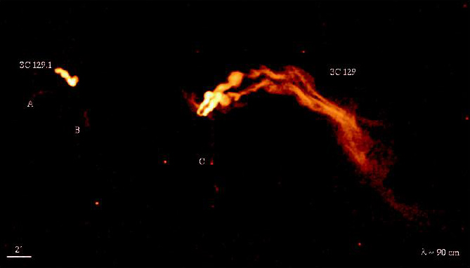
In 1968, Ryle and Windram found the first examples of a type of radio galaxies, whose radio emission extends from the optical galaxy in one direction in the form of a radio “tail” or “trail”. These examples were NGC 1265 and IC 310 in the Perseus cluster. Soon other examples were found in the Coma cluster of galaxies (NGC 4869, alias 5C4.81), as well as the radio galaxy 3C 129. The latter lies right in the plane of our Galaxy, and its membership in a cluster of galaxies was only confirmed much later, hampered by the dust obscuration of our own Milky Way. All three of these tailed radio galaxy were located close to another radio source, with their tails pointing more or less away from their radio neighbor, leading these authors to suspect that the tails were blown by winds of relativistic particles ejected from the radio neighbor. Soon thereafter higher-resolution observations of these sources revealed that the host galaxies showed the same two opposite radio jets as known from other, less bent, radio galaxies like Cygnus A, but close to the outskirts of the optical galaxies the jets would both bend in some direction, thought to be the direction opposite to the motion of the host galaxy through the so-called “intergalactic” or “intracluster” medium, which had been discovered from X-ray observations at about the same time. Later on, doubts were cast on this scenario, as it was found that the optical hosts of tailed radio galaxies in clusters did not move about within their clusters with high enough velocities to explain the bends in the jet.
VLA radio image of 3C 465
A detailed study of the prototypical WAT source 3C 465 (image above) at the center of the rich Abell cluster of galaxies A2634 by these authors did not result in any plausible explanation for the bending of their radio trails. Later on, with more detailed X-ray images of clusters of galaxies, it was found that tailed radio galaxies occur preferentially in high-density regions of the intracluster medium (i.e. where the X-ray intensity is high; for more information, see this 1994 study) and even cluster mergers were made responsible for the formation of radio tails in this 1998 study. More recently authors seem to converge on the compromise idea that the combination of high ambient density and modest speeds of the host galaxy with respect to the ambient medium are able to produce the bends, but in this blog I would rather like to concentrate on the variety of morphologies shown by these objects in order to help RGZ users to classify them.
Above all, the term “tailed radio galaxies” should never be separated from the word “radio”. Some authors talk about “tailed” or “head-tail (HT) galaxies”, but the tail always occurs in their radio emission, usually far beyond the optical extent of their host galaxies. So, let us reserve the term “head-tail galaxies” for a future when optical tails may be detected in certain galaxies. Also, please note that while galaxies sometimes show optical tails due to tidal interactions, these are of totally different origin than the radio tails we discuss here.

Arp 188, a.k.a. The Tadpole Galaxy: not a tailed radio galaxy. I repeat, not the subject of this blog post.
Tailed radio galaxies are often subdivided into wide-angle (WAT) and narrow-angle tailed (NAT) radio galaxies, referring to the opening angle between the two opposite jets emanating from the nucleus of the optical galaxy, where we expect the supermassive black hole doing its job of spewing out the jets. However, the distinction between WATs and NATs depends strongly on the angular resolution and/or the distance to the radio source. E.g., the first HT radio galaxy to be discovered (NGC 1265; images below) may be called a WAT at high resolution, but appears as a (much larger) NAT at lower resolution, shown by this sequence of high, medium and low resolution radio images:


First Result from Galaxy Zoo Hubble
Posted on behalf of Tom Melvin:
Hello everyone, my name is Tom Melvin and I’m a 3rd year PhD student at Portsmouth University. I have been part of the Galaxy Zoo team for over two years now, but this is my first post for the Galaxy Zoo blog, hope you enjoy it!
I’m very happy to bring you news of the latest paper based on Galaxy Zoo classifications, and the first paper based on Galaxy Zoo: Hubble classifications. Galaxy Zoo: Hubble was the first Galaxy Zoo project to look at galaxies beyond our local universe, using the awesome power of the Hubble Space Telescope. These images contained light from galaxies which have taken up to eight billion years to reach us, so we see them as they appeared eight billion years ago, or when the universe was less than half its current age! So what is the first use of this data? Well, we combine our Galaxy Zoo: Hubble classifications with Galaxy Zoo 2 classifications to explore how the fraction of disk galaxies with galactic bars has changed over eight billion years.
Here’s the title…..

Our work is based on a sample of 2380 disk galaxies, which are from the Cosmic Evolution Survey (COSMOS), the largest survey Hubble has ever done. To see how the bar fraction varies over such a large time-scale, we look at the number of disk galaxies and what fraction of them have bars in 0.3 Gyr (300 million year) time steps. In Figure 1 we show that eight billion years ago only 11% of disk galaxies had bars. By 4 billion years ago this fraction had doubled, and today at least one third of disk galaxies have a bar.

Figure 1: The evolving bar fraction with cosmic time (Figure 7 in the paper).
We know that bars tend to only form in disk galaxies which have low amounts of atomic gas and are in a relaxed state, or what we call ‘mature’. Combining this knowledge with our observations, we can say that, as the Universe gets older, the disk galaxy population as a whole is maturing. To see whether this is true for all disk galaxies, we split our sample up into three stellar mass bins, allowing us to look at the evolving bar fraction trends for low, intermediate and high mass disk galaxies.

Figure 2: Mass dependent evolution of the bar fraction with cosmic time (Figure 8 in the paper)
The results for this are shown in Figure 2, where we observe an intriguing result. The bar fraction increases at a much steeper rate with time for the most massive galaxies (red), compared to the lower mass galaxies (blue). From this we can say that the population of disk galaxies is maturing across the whole stellar mass range we explore, but it is predominantly the most massive galaxies which drive the overall time evolution of the bar fraction we observe in Figure 1.
At the end of the paper we offer an explanation as to why the time evolution of the bar fraction differs for varying stellar mass bins. We can make the reasonable assumption that, by eight billion years ago, the majority of massive disk galaxies have formed, and have been, and continue to form bars up to the present day – hence the steeply increasing bar fraction we observe. However, the same assumption is not true for the low mass galaxies. There are some which are ‘mature’ disk galaxies eight billion years ago, but not all are ‘mature’ enough to be classified as disks. As with the most massive galaxies, these low mass disks are forming bars at a similar rate up to the present day, but the difference with this low mass sample is that there are still low mass disks forming up to the present day as well – leading to the much shallower increase in the bar fraction with time we observe.
In addition to these results, we are also able to present an interesting subset of disk galaxies. Your visual classifications has allowed our work to include a sub-sample of ‘red’ spiral galaxies (like those found from Galaxy Zoo 2 classifications). This sub-sample is generally omitted from other works that have explored this topic, as their way of identifying disks is based on galaxy colours. This means that these ‘red’ galaxies would have been classified as elliptical galaxies! Figure 3 shows a few of these ‘red’ disk galaxies (with the full sample of 98 here), so why don’t you take a look and decide for yourself! Not only is it very cool that you are able to identify these ‘red’ disks, but they also influence the results we observe. Just like in our local universe, these ‘red’ disks have a high bar fraction, with 45% of them having a bar! Could this be a further sign that bars ‘kill’ galaxies, even at high redshifts?

Figure 3: A sample of ‘red’ disk galaxies found by Galaxy Zoo volunteers (Figure 10 in the paper).
So that is a summary of the first results from Galaxy Zoo: Hubble. If you want more detail have a read of the paper in full here and take a look at the press release too! Thanks for all your hard work and help in classifying these galaxies!
Posted on behalf of Tom Melvin.
Galaxy Zoo and undergraduate research: spiral arms, colors, and brightnesses
The guest post below is by Zach Pace, an undergraduate physics student at the University of Buffalo. Zach worked at the University of Minnesota during the summer of 2013 through the NSF’s Research Experience for Undergraduates (REU) program. Zach is continuing to work with Galaxy Zoo data as part of his senior thesis.
Hi, everyone–
My name is Zach Pace. I’m an undergraduate physics student from the University at Buffalo, and I’ve been working on the Galaxy Zoo 2 project at the University of Minnesota since late May with Kyle Willett and Lucy Fortson. My investigation has been twofold: I have been diagramming specific morphological categories in color-magnitude space, and also fitting those data to mathematical functions.
As many readers probably know, a galaxy’s magnitude (overall brightness in the red band, on a log scale) and a galaxy’s color (the difference between the blue magnitude and a red band) are two important quantities for determining what a galaxy might look like (and how it might evolve). Brighter galaxies have more mass (more stars produce more light, of course), and bluer galaxies have a more recent star formation history (this is because young, bright stars tend to be large, bright, and blue). In terms of the whole population, we know, for instance, that elliptical galaxies tend to concentrate in a red sequence, and have typical colors between 2.25 and 2.75. Conversely, the vast majority of spiral galaxies concentrate in a blue cloud between colors 1.25 and 2.0. These two populations are clearly separated in color-magnitude space (this can be seen in the accompanying 2-D histogram, made from Zoo 2 data).

Color-magnitude diagram (CMD) for objects in Galaxy Zoo 2. The lines show fits to the two main populations of elliptical (red) and spiral (blue) galaxies, following the method of Baldry et al. (2004). The green line shows an approximate separation between them.
One of the main goals of Zoo 2 is to gauge the extent to which morphology informs physical characteristics like color and magnitude, so my objective for the summer was to come up with good representations of color and magnitude for all of the smaller sub-populations in Zoo 2.
Several of my results were interesting and surprising. For instance, it has been suggested that spiral galaxies with more arms and spiral galaxies with tighter arm winding (which is to say, a shallower pitch angle) tend to be brighter and bluer. This can be intuitively understood as follows: tighter winding of spiral arms and the presence of more spiral arms indicate, on average, denser gas clouds in those arms, which is tied to increased star formation and bluer color. However, I wasn’t able to measure this in the Zoo 2 data (all the differences were on the order of the histograms’ bin size, about 0.1 magnitude, or about a 10% difference in brightness). This suggests that spiral galaxies, no matter arm multiplicity or winding, are drawn from the same base population.

Color-magnitude diagram (CMD) for spirals in GZ2, split by the number of spiral arms identified in each galaxy. The distribution of colors and magnitudes for galaxies are statistically similar, no matter what the number of spiral arms.
I also came across something unexpected when looking at bulge sizes in face-on disk galaxies. The distribution of galaxies classified by users as bulgeless is starkly different from the distribution of obvious bulge and bulge-dominated galaxies. Furthermore, the population with a bulge that is just noticeable seems to form an intermediate population between the bulgeless and bulge. This observation is also borne out in edge-on disk galaxies: the population of bulgeless edge-on galaxies has a similar shape to the population of face-on galaxies, albeit with stronger reddening on the bright end.

Color-magnitude diagram (CMD) for disk galaxies in Galaxy Zoo 2, split by the relative size of the central bulge. Galaxies that appear to have no central bulge (top) have very different colors and luminosity than those with dominant bulges (bottom).
To fit the distributions, I used a method pioneered about 10 years ago by Ivan Baldry, which fits one parameter after another in our profile functions to find a distribution that converges onto the best fit. It works okay (but not great) for the whole sample, and it fails pretty badly when working with the smaller sub-populations. This is because I have to fit many parameters at once, and do that a bunch of times in a row for the fit to converge, so there are a lot of points of failure. I’m working now at Buffalo towards finding a different and better fitting routine, which will allow us to represent more distributions mathematically.
If you have any questions, feel free to comment below.
