
Next GZ Hangout: 3rd of September, 3 pm GMT
The hangouts have returned from a midsummer hiatus! Our next hangout will be Tuesday, September 3rd, at 3 pm GMT. That’s 8 am PDT, 11 am EDT, 4 pm BST, 5 pm CET, 6 pm CAT. Unfortunately I think that’s 11 pm in Japan and midnight in Sydney, but hopefully we’ll have a hangout at a different time very soon!
Just before the hangout we’ll update this post with the embedded video, so you can watch it live from here. If you’re watching live and want to jump in on Twitter, please do! we use a term you’ve never heard without explaining it, please feel free to use the Jargon Gong by tweeting us. For example: “@galaxyzoo GONG dark matter halo“.
In the meantime, please feel free to leave a question in the comments below. See you soon!
Update: read a summary of the Hangout here: What is a Galaxy?… the Return
Quench Boost: A How-To-Guide, Part 2
It was amazing how quickly the new Quench classifications were completed. We posted them on Friday and you were already done by Sunday morning. Wow, that’s awesome! This means we can turn our full attention to making sense of the data. And we need your help!
In Part 1 of this How-To-Guide to data analysis within Quench, you learned how to use Tools, our analysis platform, and were inspired (or so I hope) about ways to play with the data as you read the background literature about post-quenched galaxies and galaxy evolution.
In Part 2 of this How-To-Guide, we’re going to help you navigate using Tools to compare results from galaxies *you* classified with the rest of the post-quenched galaxy sample.
You’re 12 small steps away from your first comparison plot between your galaxies and the full sample… let’s get started!
Step 1: Enter Tools and log in using your Zooniverse login information.
Step 2: Choose ‘Quench’ in the pull-down menu in the upper-left, next to the words ‘zootools’. Now click ‘Create Dashboard*’ in the upper-right, and give it a name, like: ‘My Data in Context’.
Step 3: Click ‘Data’ in the upper-left and choose ‘Zooniverse’ in the pop-up options.
Step 4: In the window that pops up, choose ‘Recents’ or ‘Collections’. Your choice.
If you classified galaxies in quench.galaxyzoo.org, they’ll be accessible through ‘Recents’. Choose the max number possible. If you created a Collection of interesting galaxies in Quench Talk or want to look at someone else’s Collection, you can access them by clicking ‘Collections’.
I’ve created a Dashboard* in Tools called ‘Example: My Data in Context’. Take a look and, if you’d like, you can even make edits by copying it into your Tools environment.
In my Dashboard ‘Example: My Data in Context’, I chose ‘Collections’. I love #Quencher SUMO_2011’s Collection of ‘Blue’ galaxies from Quench. If you go to that URL, the Collection ID is listed after the final ‘/’ in the URL. In this case, the Collection ID is CGSS00000x. I inputted that ID into the pop-up window in Tools, in the box next to ‘Enter Collection Id:”. I then clicked on ‘Import Data’.
Step 5: Now that you have your galaxies’ information imported into the Dashboard, it’s time to play with them. Click on ‘Tools’ in the upper-left and choose ‘Table’ in the pop-up options.
Step 6: In your Table window, choose ‘Zooniverse-1’ in the pull-down menu under ‘Data Source’. Now the Table knows to work with that set of data.
Step 7: As in Part 1 of this How-To-Guide (https://blog.galaxyzoo.org/2013/08/23/quench-boost-a-how-to-guide-part-1/), you’ll make a new column that has color information about your galaxies. You do this by subtracting the brightness of your galaxy in one filter from the brightness of your galaxy in another filter.
In the open space under ‘Prompt’ in your Table, write: field ‘My Galaxies Color u-r’, .u-.r
If you scroll to the right in your table, you’ll see that you created a new column of information, called ‘My Galaxies Color u-r’.
Step 8: Click ‘Tools’ in the upper-left and choose ‘Scatterplot’ in the pop-up options.
Step 9: In your Scatterplot window, choose ‘Table-2’ in the pull-down menu under ‘Data Source’. Now the Scatterplot knows to work with the Table, which includes your new column with Color information.
Step 10: Choose ‘log_mass’ for the X-axis and ‘My Galaxies Color u-r’ for the Y-axis. Recent star formation is seen strongly in the u-band while older stars dominate the r-band. The color, u-r, tells you about the star formation history for each of your galaxies. Check out this post for more details.
Step 11: How do your galaxies compare with the full sample of post-quenched galaxies? To answer this, we redo the steps 3-10 above, but for the post-quenched galaxy sample.
- Click on ‘Data’ in the upper-left and choose ‘Quench’ in the pop-up options.
- Click on ‘Quench Sample’ in the pop-up window.
- Click on ‘Tools’ in the upper-left and choose ‘Table’ in the pop-up options.
- In the new Table window, choose ‘Quench-4’ in the pull-down menu under ‘Data Source’. This loads the Quench Sample into that Table.
- In the open space under ‘Prompt’ in your Table, write: field ‘Quench Galaxies Color u-r’, .u-.r
- Click on ‘Tools’ in the upper-left and choose ‘Scatterplot’ in the pop-up options.
- In the new Scatterplot window, choose ‘Table-5’ in the pull-down menu under ‘Data Source’.
- Choose ‘log_mass’ for the X-axis and ‘Quench Galaxies Color u-r’ for the Y-axis.
- Zoom in on the data, for example, choosing Xmin: 7, Xmax: 12, Ymin: 1, and Ymax: 4.
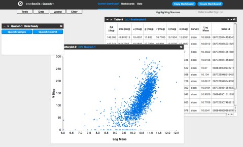
Step 12: Place your two scatterplots side by side. For a fair comparison, make sure the x- and y-axis range is the same for both plots, otherwise the stretch might skew your analysis. I tend to make the axes ranges in the plot showing My Galaxies match the plot showing the Quench Sample.
What do you notice about your subsample of post-quenched galaxies compared to the full sample? Do they occupy a particle sub-space within the plot? Or are they randomly distributed throughout the quench space?
The figure below shows what you’ll see if, like me, you uploaded SUMO_2011’s Collection of blue galaxies. You’ll notice that all of the blue-collection galaxies are way bluer (closer to the bottom of the plot, near values u-r = 1.5) than the full post-quenched galaxy sample (which spread from u-r values of 1 to u-r values of 3.5 and higher). This is a reassuring reality check given what you see visually when you look at the color of the galaxies. The plot also tells us that since these blue galaxies have such low values of ‘u-r’, they’ve had more recent star formation than most of the post-quenched galaxies.
In looking at these two plots side-by-side, I wondered: Why are there so few massive post-quenched galaxies (log_mass > 11) with bluer colors (u-r < 2.0)? If we compare our post-quenched galaxies with our control galaxies, do I see any difference? Specifically, are there massive (log_mass > 11) control galaxies with bluer colors (u-r < 2.0)? If there are, what might that be telling me about our post-quenched galaxy sample?
Stay tuned for Part 3 of our How-To-Guide for taking part in the analysis phase of the research process. If you have suggestions for what you’d like to learn more about, please post here. Thank you all, and keep on Quenching!
*Dashboard is the place within Tools (tools.zooniverse.org) for volunteers to observe, collect, and analyze data from Zooniverse citizen science projects.

Quench Boost: A How-To Guide, Part 1
The reaction to GZ Quench has been amazing. It has been great to see the interest and enthusiasm for supporting citizen scientists in experiencing the full scientific process.
This morning’s post was about how we have a small sample of additional galaxies to classify. I’ve really enjoyed watching how fast those are being done… gotta love the counter at http://quench.galaxyzoo.org/. Thank you all!
This post is Part 1 of our How-To-Guide for analyzing our classification results. It’s clear that you’re interested in getting your analysis on, but it may be that you’re not sure where to start. That’s 100% understandable and we’re here to help. We’ve broken down the steps into bite-size chunks. Let’s get started.
The first thing to do is to meet Quench Tools. This is the web platform to help you play with the data. To enter Quench Tools, click here. An in-line Tutorial will automatically pop-up, and guide you through entering the Quench area, loading the data, and creating your first figure. For additional information about Tools, check out our GZ Hangout about Tools, our text-based Tools Tutorial, and this Quench Talk discussion forum post.
In parallel with getting to know Tools, you may be interested in understanding the science context for why post-quenched galaxies (the GZ Quench sample) are so interesting for galaxy evolution studies. A great starting place for getting a sense of the science context and motivation is to read the summaries (written for the general public) of science articles at http://postquench.blogspot.com/. It’s modeled after the astrobites blog, a great resource for any astronomy enthusiast!
As you read those posts, you might want to join the conversation within the Quench Talk discussion forum. There are also a slew of links to popular science articles and websites for additional information about post-quenched galaxies and galaxy evolution.
And if you feel it would help to take a step back and see the big picture, definitely check out our initial GZ Quench blog post and this Quench Talk post.
Stay tuned for Part 2 of our How-To-Guide. In it, I’ll guide you through the next bite-size piece of this adventure – playing with your own classification results!
Quench: New Classifications Needed
We have a few dozen new galaxies in GZ Quench that need your classification savvy. As with all research projects, there are sure to be some glitches. Luckily we have a great group of Quenchers on the job. And as a few pointed out (including the force of nature that is Jean Tate!), 57 of our 3002 control sample galaxies were duplicates. We’ve identified suitable replacements and, to make sure no bias is introduced, we’ve added some of the original post-quenched galaxies to the mix as well. So let’s get classifying!
For a reminder about what GZ Quench is all about, check out the first Quench blog post. Yes, in this project, we’re not only classifying galaxies, but we’re going all the way to support our citizen scientists in experiencing the full process of science.

We’re now into Phase 2 of GZ Quench, analyzing the results of the classifications and making sense of our data. Our amazing group of Quenchers have provided incredibly useful feedback on the analysis tools we’ve made available and the analysis process. And there are already a number of intriguing results (for example, here and here)!
We’re now ready to give Quench a boost. Later today I’ll post Part 1 of our How-To-Guide, breaking the analysis phase into bite-size pieces and providing a smoother on-ramp for all of you out there who want to join in the GZ Quench experience, but aren’t sure where to begin.
Stay tuned…
GZ: Quench data update
Since finishing the classifications for the GZ: Quench project, many of our volunteers have been analyzing that consensus data using the tools at tools.galaxyzoo.org. We made a few changes to the site earlier this week, and I’d like to describe them and talk about how it might affect your work on the project.
First, a quick reminder of how the data is presented. As most of you probably remember, the classification process on GZ: Quench (and all GZ projects since GZ2) is what we call a “decision tree”. We begin with a broad question on morphology (ie, “Is this galaxy smooth, or does it have features or a disk?”) for the volunteer to answer. We then ask more specific follow-up questions that depend on the previous answers. For example – if you said the galaxy doesn’t have any spiral arms, it doesn’t make sense for us to then ask you how many arms there are – it doesn’t apply to this galaxy! So, out of 11 potential questions covering galaxy morphology, a single classifier will only answer a subset (between 4 and 9) of them. Here’s a flowchart of the decision tree for GZ: Quench — it’s an interesting exercise to look at it and work out how many unique morphologies you could sort galaxies into by going through the tree.

Flowchart of the morphology decision tree for GZ: Quench
So, why this discussion? When we added the data to the Tools website, we added a label in each category that gave the most common response to that question. For example, under “Arm tightness”, you could see that all galaxies were either “Tight”, “Medium”, or “Loose”. However, this is problematic when you’re trying to analyze data and compare different sets of galaxies. For smooth (or elliptical) galaxies, though, this arm classification is the result of very few votes (or even none) — they don’t represent the majority of classifications, and thus we really shouldn’t be including them when trying to compare what makes a medium-wound vs. a loosely-wound spiral.
The solution we’ve adopted has been to edit the data on Tools — questions whose answers don’t apply to the consensus morphology (eg, spiral arms in a smooth galaxy, or the roundness of a spiral) are now blank. This means that if you look at the average color or size of any of these morphology properties, you’re now truly comparing similar groups of objects (apples to apples). Including other galaxies in earlier samples likely introduced a significant amount of bias – the science team thinks that this will largely help to address that.
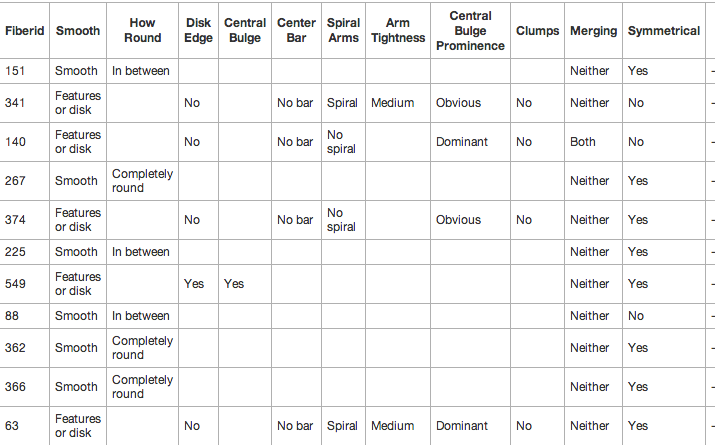
Example of the new GZ: Quench classification set in Tools
What does this mean for your analysis? Most of your old Dashboards and results should still work and remain valid results. For any work where you were analyzing morphological details (especially for spiral structure), though, we encourage you to revisit these and run them again on the new, filtered dataset. Please keep posting any questions you have on Talk, and we’ll answer them as soon as we can. Good luck!
Galaxy Zoo 2 data release
It’s always exciting to see a new Galaxy Zoo paper out, but today’s release of our latest is really exciting. Galaxy Zoo 2: detailed morphological classifications for 304,122 galaxies from the Sloan Digital Sky Survey, now accepted for publication in the Monthly Notices of the Royal Astronomical Society, is the result of a lot of hard work by Kyle Willett and friends.

Lead author Kyle, seen here taking a rare moment away from reducing Galaxy Zoo data.
Galaxy Zoo 2 was the first of our projects to go beyond simply splitting galaxies into ellipticals and spirals, and so these results provide data on bars, on the number of spiral arms and on much more besides. The more complicated project made things more complicated for us in turning raw clicks on the website into scientific calculations – we had to take into account the way the different classifications depended on each other, and still had to worry about the inevitable effect that more distant, fainter or smaller galaxies will be less likely to show features.
We’ve got plenty of science out of the Zoo 2 data set while we were resolving these problems, but the good news is that all of that work is now done, and in addition to the paper we’re making the data available for anyone to use. You can find it alongside data from Zoo 1 at data.galaxyzoo.org. One of the most rewarding things about the project so far has been watching other astronomers make use of the original data set – and now they have much more information about each galaxy to go on.
And the winner is….. Arp 142 (The Penguin Galaxy)
Well it was a very close fought battle, but the winner of our fun vote to pick the cover image for the October A&G was:
Apr 142 (aka The Penguin Galaxy):

I include below a screen shot of the poll from today, which confirms that choice. We have now sent this choice to the cover editor, so we won’t count any more votes.

(Most) Galaxy Zoo Papers now Open Access
As announced on the Zooniverse blog, Oxford University Press have agreed that to make the Zooniverse papers published in Monthly Notices of the Royal Astronomical Society open access. While they’ve always been freely available on astro-ph, it’s nice that everyone who contributed can now get access – for free – via the main journal site.
GZ Quench: Classification Complete – Now the Real Fun Begins!
Congratulations all! We’ve completed Phase 1 of Galaxy Zoo Quench! Over 1600 people lent us their time and pattern-recognition skills to complete the needed 120,000 classifications. Thank you!
Now is when GZ Quench gets really fun, interesting, and totally different from past projects. We’re not stopping with classifications; we’re helping our volunteers to go all the way… from soup to nuts, as some like to say.
Phase 2 begins today and will run for the next few weeks*, with our science team supporting you, our esteemed Zooniverse volunteers, in the data analysis and discussion.

We’ll be using the results from our classifications of the 3002 post-quenched galaxies + 3002 control galaxies to address the following questions: What causes the star formation in these galaxies to be quenched? What role do galaxy mergers play in galaxy evolution? Join us in exploring these questions, being a part of the scientific process, and contributing to our understanding of this dynamic phase of galaxy evolution!
Luckily, we have great tools to help make this phase accessible to anyone, no matter your background.
- Quenchtalk.galaxyzoo.org – our discussion forum within which there are already really interesting and exciting conversations happening between Zooites and the science team. This forum allows us to share knowledge, pursue interesting results, collaboratively make sense of interesting plots, and determine which results to include in our article.
- Tools.zooniverse.org – our online data visualization environment, which helps you play with the data and look for trends. Click here for the blog post and to watch the GZ google hangout describing Tools and the Quench Tools tutorial.
- Authorea.com – the online article writing platform we’ll be using to collaboratively write the GZ Quench article, to be submitted to a professional journal. This is the same online environment that a group of over 100 CERN physicists are using to write their articles.
We can’t stress enough that you do not need prior background or knowledge to take part in this next phase. Each of you brings useful skills to the project – asking questions, communication, critical thinking, organization, leadership, consensus building, intuition, etc. Through Quench Talk, we’ll help you apply those skills in this context, and enable you to get your feet wet experiencing the full process of science.
Have questions about the project? Ask us on Twitter (@galaxyzoo), Facebook, or within Quench Talk.
*Science timelines often subject to a factor of two uncertainty. We’ll do our best to keep on track, at the same time expecting the unexpected (all part of the fun of doing science!).
Using Galaxy Zoo Classifications – a Casjobs Example
As Kyle posted yesterday, you can now download detailed classifications from Galaxy Zoo 2 for more than 300,000 galaxies via the Sloan Digital Sky Survey’s “CasJobs” – which is a flexible SQL-based interface to the databases. I thought it might be helpful to provide some example queries to the data base for selecting various samples from Galaxy Zoo.
This example will download what we call a volume limited sample of Galaxy Zoo 2. Basically what this means is that we attempt to select all galaxies down to a fixed brightness in a fixed volume of space. This avoids biases which can be introduced because we can see brighter galaxies at larger distances in a apparent brightness limited sample like Galaxy Zoo (which is complete to an r-band magnitude of 17 mag if anyone wants the gory details).
So here it is. To use this you need to go to CasJobs (make sure it’s the SDSS-III CasJobs and not the one for SDSS-I and SDSS-II which is a separate page and only includes SDSS data up to Data Release 7), sign up for a (free) account, and paste these code bits into the “Query” tab. I’ve included comments in the code which explain what each bit does.
 -- Select a volume limited sample from the Galaxy Zoo 2 data set (which is complete to r=17 mag).
 -- Also calculates an estimate of the stellar mass based on the g-r colours.
 -- Uses DR7 photometry for easier cross matching with the GZ2 sample which was selected from DR7.
 -- This bit of code tells casjobs what columns to download from what tables.
 -- It also renames the columns to be more user friendly and does some maths
 -- to calculate absolute magnitudes and stellar masses.
 -- For absolute magnitudes we use M = m - 5logcz - 15 + 5logh, with h=0.7.
 -- For stellar masses we use the Zibetti et al. (2009) estimate of
 -- M/L = -0.963+1.032*(g-i) for L in the i-band,
 -- and then convert to magnitude using a solar absolute magnitude of 4.52.
 select g.dr7objid, g.ra, g.dec,
 g.total_classifications as Nclass,
 g.t01_smooth_or_features_a01_smooth_debiased as psmooth,
 g.t01_smooth_or_features_a02_features_or_disk_debiased as pfeatures,
 g.t01_smooth_or_features_a03_star_or_artifact_debiased as pstar,
 s.z as redshift,
 s.dered_u as u, s.dered_g as g, s.dered_r as r, s.dered_i as i, s.dered_z as z, s.petromag_r,
 s.petromag_r - 5*log10(3e5*s.z) - 15.0 - 0.7745 as rAbs,
 s.dered_u-s.dered_r as ur, s.dered_g-s.dered_r as gr,
 (4.52-(s.petromag_i- 5*log10(3e5*s.z) - 15.0 - 0.7745))/2.5 + (-0.963 +1.032*(s.dered_g-s.dered_i)) as Mstar
-- This tells casjobs which tables to select from.
 from DR10.zoo2MainSpecz g, DR7.SpecPhotoAll s
-- This tells casjobs how to match the entries in the two tables
 where
 g.dr7objid = s.objid
 and
 -- This is the volume limit selection of 0.01<z<0.06 and Mr < -20.15
 s.z < 0.06 and s.z > 0.01
 and (s.petromag_r - 5*log10(3e5*s.z) - 15 - 0.7745) < -20.15
--This tells casjobs to put the output into a file in your MyDB called gz2volumelimit
 into MyDB.gz2volumelimit
Once you have this file in your MyDB, you can go into it and make plots right in the browser. Click on the file name, then the “plot” tab, and then pick what to plot. Colour-magnitude diagrams are interesting – to make one, you would plot “rabs” on the X-axis and “ur” (or “gr”) on the yaxis. There will be some extreme outliers in the colour, so put in limits (for u-r a range of 1-3 will work well). The resulting plot (which you will have to wait a couple of minutes to be able to download) should look something like this:

Or if you want to explore the GZ classifications, how about plotting “psmooth” (which is approximately the fraction of people viewing a galaxy who thought it was smooth) against the colour.
That plot would look something like this:
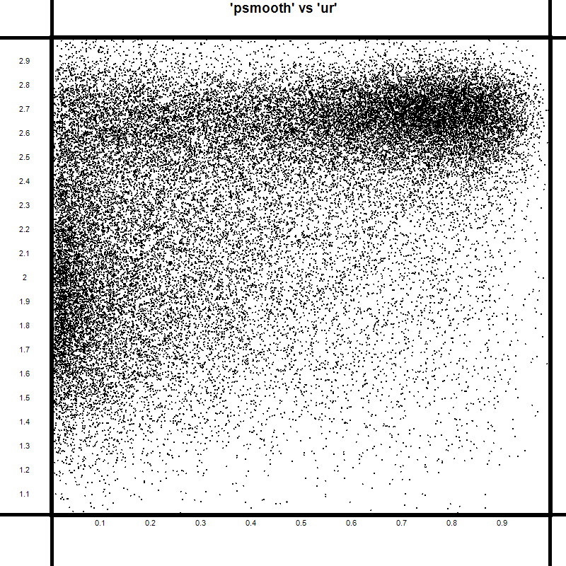
Which reveals the well known relationship between colour and morphology – that redder galaxies are much more likely to be ellipticals (or “smooth” in the GZ2 language) than blue ones.
You can learn more about SQL and the many things you could do with CasJobs at the Help Page (and then come back and tell me how simple my query example was!).
This example only downloads the very first answer from the GZ2 classification tree – there’s obviously a lot more in there to explore.
(Note that at the time of posting the DR10 server seemed to be struggling – perhaps over demand. I’m sure it will be fixed soon and this will then work.)
